The main data source is a collection of loan-listing web pages from PPDai.com. The data were obtained by downloading all the loan-listing web pages since the platform’s official inception (June 2007 to October, 2015). Next, a pattern-matching algorithm was listings submitted by more 3.9 million potential borrowers, among which 98,1629 loan listings were funded, and investment track records of more than 140,000 individual investors. Items with nonstandard or missing data were disregarded, and earlier and later data were discarded to avoid the initial launch period and truncation on loan repayments. The period studied is from November 2011 to October 2015, which comprise a four-year interval.
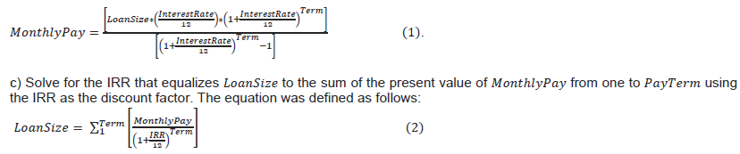
The IRR of the defaulted loans was calculated using the approach of Freedman and Jin (2014). If a loan is not defaulted, then the IRR is equal to the interest rate of the loan, because loans with truncation on loan repayments were disregarded in the interval studied. The detailed algorithm is as follows:
a) Loan size ( ), interest rate of a loan ( ), term to amortize ( ), and number of months during which the payments have been made ( ) were determined.
Given a loan without any payment or defaulted at the first month, we set the = -12, and = 1, which means that the monthly
discounter factor is -1. The dataset allows us identify the investment decisions made by individual investors or the platform. The rate
s of return of individual investors and platform was calculated independently. We can calculate the rates of returns on a portfolio in week given a portfolio that contains bids in week because the , , and (amount of bid) for each bid is known. The rates of returns are calculated as follows:

Five additional rate-of-return series are calculated as representations of the investment performance of the benchmark “market” collections of loans. According to PPDai.com, the loans are aggregated into the following types: loans with low risk by default (loans assigned with credit grade “AAA” or “AA”), loans with middle risk by default (if credit grade of the loan is “A”, “B” or “C”), and loans with high risk by default (which are graded into “E” or “F”).
A type for loans that have the lowest risk by default (loans graded into “AAA”) was added. These types (“low risk,” “middle risk,” “high risk” and “safe risk”) and the four portfolios (low risk, middle risk, high risk and safe risk) are constructed from the four types of loans. Based on Expression (3), the rate-of-return series of all these portfolios are obtained. The November 2011 to October 2015 weekly rates of return correspond to the low-risk portfolio, middle- risk portfolio, high-risk portfolio, safe-risk portfolio and market implemented to take the variables of interest from the web page HTML code. The resulting dataset consists of more than 5 million portfolio. Given that one of the objectives of this study is to examine the investment performance of individual investors, we do more than just measure the average return of individual investors. Moreover, the proportions of investors who outperform the market and underperform the market must be determined. This information can be obtained from two aspects, namely, total investment size and investment experience. Investment experience is measured by the number of weeks an investor bids on some loan listings. For example, if an investor funds loan listings in two distinct weeks, the investment experience of the investor is equal to two. These two criteria were chosen mainly because of the following reasons. A less-sophisticated investor tends to obtain a low or negative return and is more likely to withdraw from the market. As a result, less skilled investors are inclined to have a small total investment size and to be less experienced from an ex post perspective. Thus, a feasible method may be employed to distinguish investors with investment skills from those with less skills. This approach involves dividing the investors into different groups according to their total investment size or investment experience. The overall performance of these groups was assessed.
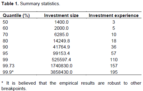
The investors must be divided into different groups to examine their performances. However, the total investment size of individual investors is heavily skewed in the dataset, as shown in Table 1. Investors below the 50th percentile have a total investment size less than RMB 1400, whereas investors in the 99.9th percentile invested more than RMB 3.8 million in the market. To avoid possible biases, we classify the investors into 10 groups and a portfolio is constructed based on each group. According to Expression (3), a rate-of-return series is calculated for each portfolio. 10 groups of investors were obtained according to the following breakpoints: bottom 50, 50-60, 60–70, 70–80, 80–90, 90–95, 95–99, 99.73–99.9 and top 99.9–100%. The same breakpoints were also set when we divided the investors according to the investment experience. The investment experience is also heavily skewed. The summaryized statistics al results are shown in Table 1. The table shows that 50% of the investors in the dataset have an investment experience not longer than a month, whereas investors in the 99.9th percentile bid on some loan listings almost throughout the four-year interval.
The attributes of the rate-of-return series of different portfolios are summarized in Table 2. Panel A shows the details of the rate-of-return series of the portfolios, which are constructed from different investment track records of various groups of investors. The arithmetic mean annualized weekly return on the portfolio of the investors below the 50th percentile during the four years is estimated to be 0.074, whereas the return on the portfolio of individual investors in the 99.9th percentile is estimated to be 0.118. A negative relation exists between the investment size of investors included in the portfolio and the standard deviation of the returns on the portfolio. A stronger positive relation exists between the total investment size of investors and the average return on the portfolio. These findings indicate that investors with a large total investment size will likely obtain high and steady returns. This phenomenon is also discovered when the performance of investors is analyzed according to their investment experience. Investors with a short investment experience will likely have low returns with a high standard deviation. This preliminary examination indicates that some individual investors outperform other investors systematically.
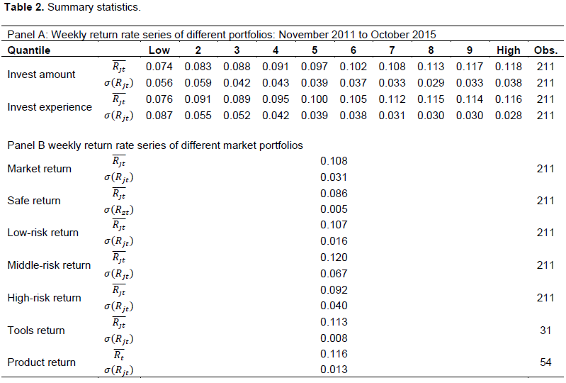
Panel B shows the details of the rate-of-return series of the benchmarks. The average return on the market portfolio is 0.108 with a standard deviation of 0.03. The average return on the safe-risk portfolio is 0.086, whereas the figure of the standard deviation is 0.005, which is significantly smaller than that of the market portfolio at 0.03. The unreported results indicate that when the weekly returns on the safe-risk portfolio are regressed on the returns of the market portfolio by OLS, the statistic of the linear regression model is close to zero, which indicates that the returns on the market portfolio slightly affect the returns on the safe-risk portfolio. The returns on the safe-risk portfolio are independent from the returns on the market portfolio. Thus, the portfolio is almost a zero-beta portfolio (Blume and Friend, 1973), which will be used in one of the empirical models.
Panel B indicates that significant differences exist in the rate-of-return series on the three portfolios consisting of loans with different risk grades (low risk, middle risk, and high risk). The average returns of the portfolios range from 0.107 for the low-risk portfolio to 0.120 and 0.092 for the high-risk portfolio with a standard deviation of 0.016, 0.067, and 0.040, respectively. The attributes of rate-of-return series of the three portfolios vary significantly. Based on the concept of Fama and French (1993), the high returns on some portfolios may incur high-risk factors. Some individual investors obtain low returns simply because of their risk preferences. For example, when an investor only bids on the loan listings with risk grade “AAA” on the average, he or she can expect a return rate of 0.086. Another investor can expect a return of 0.107 if he or she also bids on loan listings with risk grade “AA” or “A”. Thus, we should employ an asset-pricing model to cover the differences of returns resulting from risk preferences. The average return on the high-risk portfolio is less than that on the middle-risk portfolio and even on the low-risk portfolio. This condition can result from the high default rate of high-risk loans. As a result, only few of the high-risk loan listings are successfully funded. The return rate of the low-risk portfolio is almost equal to the return rate of the market (0.108) but with a substantially small standard deviation. This descriptive statistical analysis indicates that funding the low-risk loans is a good choice.
The rates of returns on the portfolios of different types of re-intermediation are also presented in Panel B. The average returns on the portfolios of investment tools and financial products are 0.113 and 0.116, respectively, and the standard deviations are 0.008 and 0.013, respectively. Meanwhile, during the same period, the average returns of the market are 0.1156 and 0.1153, and the standard deviations are 0.0074 and 0.0075, respectively. The difference between the rate-of-return series is almost negligible. Hence, the re-intermediation, such as investment tools and financial products, can hardly overcome outperform that of the market. Nevertheless, these tools types of “re-intermediation” can help individual investors obtain a return rate that is not lower than that of the market.
Risk-adjust performance criteria
However, a rigorous and complete appraisal of performance results requires that the differences in investment risk preferences be considered as well and additional benchmarks be constructed. The asset pricing models of Sharpe (1964), Black et al. (1972), Merton (1973) and Fama and French (1993) can be used to organize ideas. A new asset pricing model was not proposed but employ asset pricing models to compare the rate-of-return series of different portfolios constructed in the previous section. To ensure the robustness and comprehensiveness of the empirical results, we run the regressions by choosing different asset-pricing models. The estimating equations have the following forms:
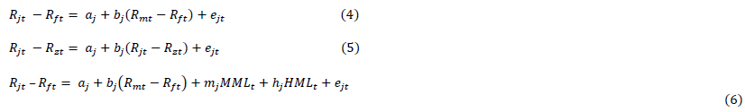
Where is the return on an individual-related or re-intermediation-related portfolio in week . is the “risk-free” rate. The one-year deposit rate of China is used as the “risk-free” rate in place of the rate of Treasury bills observed at the beginning of week . is the return on the safe-risk portfolio (consisting of loans with risk grade AAA) in week , and (middle minus low) is the difference in each week between the return on the middle-risk portfolio (consisting of loans with a middle risk grade) and the return on the low-risk portfolio (consisting of loans with low-risk grade). (high minus low) is the difference of each week between the return on the high-risk portfolio (consisting of loans in the high-risk grade) and return on the low-risk portfolio. is the error term and the regression yield parameter , , , . The estimate of intercept provides a measure of portfolio ’s risk-adjusted performance over a concerned period and a measure of the volatility on coefficient . If estimate is statistically and significantly positive, the portfolio obtains a positive excess return and outperforms the benchmark. If estimate is statistically significant and larger than 1, the volatility of the portfolio is higher than that of the market or vice versa. The return performance of different portfolios of interest is assessed through the following steps. Equation was examined by using the excess return of market, to explain the excess returns of the portfolios of interest. Equation uses as an explanatory variable, and we utilize as the “risk-free” rate. Equation uses , , to explain the excess returns on an individual-related or re-intermediation-related portfolio .
The process of computing Equation , which is the base model or building block, is similar to the approach of Sharpe (1964) and only obtains the market factor. We construct estimating Equation by re-defining the “risk-free” rate and choosing the rate of return on the safe-risk portfolio as the “risk-free” rate, because the influence of the rate of return on the market portfolio is low or is, in other words, a zero-beta portfolio. The model is a two-factor version of the market model, which is consistent with the work of Blume and Friend (1973) and was also adopted by Schlabraum et al. (1978a). Estimating Equation considers the systematical risk of the market and the risk resulting from loans with different credit grades. The previous analysis shows that the rate-of-return series on portfolios consisting of loans with different risk grades varies significantly. Estimation of Equation 3 was used to handle these differences.
Performance of individual-related portfolios
Can larger investors make an excess return?
The investigation is conducted by examining the performance of investors according to the total investment size. The parameters of the three equations are estimated from time series regressions utilizing the 211 weekly return observations available from the four-year interval. The results of these regressions are reported in Table 3.
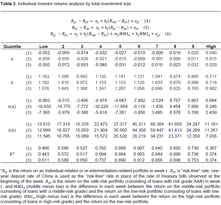
The estimate changes from negative to positive and is statistically significant (29/30) in most of the regression results, which indicates that investors with a large total investment size will likely obtain an excess return because is the measure of the portfolio’s risk-adjusted performance. However, estimate decreases gradually, indicating that the returns of investors with a large investment size are less affected by the market when compared with investors with a small total investment size, or, in other words, the volatility of the rate-of-return series of investors with a large investment size is lower. These results are consistent with the summaryized statisticasl of the rate-of-return series results in Table 2. ranges from 0.367 to 0.956. In some cases, our models attribute the relatively large common variations to other possible factors, which cannot be captured in our model. Nevertheless, the average statistic is equal to 0.7068, which ensures the reliability of our conclusions. The values in the estimated results of Equation are larger than those of Equations and , whereas the differences are almost negligible. The robustness of the empirical results may also be ensured, suggesting that the risk preferences influence investment performance, although the effect is quite limited.
The results show that estimate is consistently negative and different from zero statistically significant when the rate-of-return series belong to the portfolios of investors below the 90th percentile. The smallest figures in the regression results from the three equations are -0.069, -0.039, and -0.092, respectively. Estimate of the portfolios of investors in the 99 to 100th percentile is consistently positive and statistically significant. The largest estimate in the estimation results of the three equations is 0.040, 0.015 and 0.032, respectively. The difference of the “excess return” between the different groups is quite large and far from negligible. The rates of return are annually calculated.
Can more experienced investors make an excess return?
Table 4 reports the estimation results of the rate-of-return series on the portfolios of investors with different investment experiences, which is similar with the previous analysis. Estimate becomes positive as investment experience increases, and estimate becomes lower than 1, suggesting that experienced investors will likely obtain an “excess return” and less volatile rates of return.
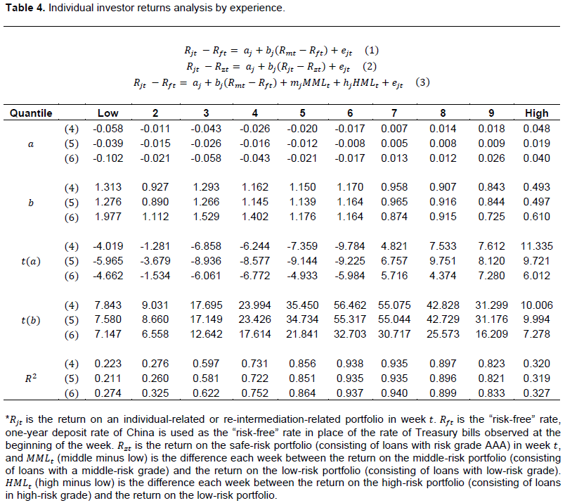
In most estimation results, the values in the estimation results of Equation are larger than those in Equations and , which are consistent with the results in Table 3. The average value of all the estimate results is 0.663. The smallest figures of estimate in the regression results from the three equations are -0.058, -0.039 and -0.102. The largest values of estimate in the results of the three equations are 0.048, 0.019 and 0.040, respectively, and the differences between these figures and those in Table 3 are almost negligible. However, Table 4 indicates that estimate is positive and statistically significant in the estimation results of the portfolios of investors over the 95th percentile. The figures in the estimation results of Equations 41 and 52 from the portfolios of the investors in the 90th to 95th percentile are equal to 0.007 and 0.005, respectively, which are not far from 0, whereas it increases to 0.013 in the regression results of Equation 63. When compared with the corresponding estimated in Table 3, the differences between estimate are relatively small. The figures are -0.005, -0.001, and 0.010, respectively, as shown in Table 3. The empirical results in Table 4 are consistent with that in Table 5 in most situations.
Performance of the re-intermediation-related portfolios
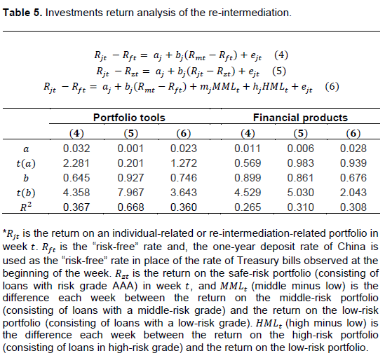
As described above, PPDai.com developed the portfolio tools to help the investors to bid on loan listings automatically. Another type of re-intermediation is the financial products provided by the platform, the financial products are managed by the platform, and the platform make investment choices Some loan listings are also funded independently of individual investors. Both approaches, which are employed by the majority of P2P lending platforms all over the world, are considered as different types of re-intermediation in this paper and the performance of them are analyzed. Firstly, the rate-of-return series was calculated on the two different portfolios of the portfolio tools and the financial products, respectively, and then the same time-series-regressions method is employed to measure the performance of these portfolios. The results of such regressions are presented in Table 5.
The performance return of the portfolio tools was first examined. Table 5 indicates that the values of estimate in the three models are 0.032, 0.001 and 0.023, respectively. The figures are positive, but estimate is only statistically significant in the estimation results of Equation 4. Concluding that portfolio tools help individuals obtain a better return than the market is unreliable. However, estimate in the three models is smaller than 1, which indicates that the return of portfolio tools may not outperform the market but obtains an average and more stable return than the market.
The performance record of the financial products managed by the platform is statistically indistinguishable from that of the indicated market benchmarks. This result is not surprising because of the close similarities of the various rate-of-return series involved. Table 5 shows that estimate has not been statistically significant for the period. Neither superior nor inferior over-all performance can be detected in these returns. Nevertheless, estimate in the three models is not larger than 1, suggesting that the returns on the financial products are less risky.