Trade liberalisation in South Africa

The South African trade policy was mainly geared towards import substitution before 1970s according to Bell (1992, 1997).  From then, quantitative restrictions started to reduce until South Africa joined the World Trade Organisation in 1994. Since then, the country reduced most of its tariffs except for agricultural commodities, textile and the automobile sector.

Most of the Computable General Equilibrium models (CGE) applied to South Africa deal with trade issues. Gelb et al. (1992) developed a dynamic one sector CGE to evaluate the impact of a negative external shock and the setting of a program of government stimuli. Then, Van der Mensbrugghe (1995, 2005), Devarajan and Van der Mensbrugghe (2000) developed a CGE to understand the impacts of trade liberalisation and increases in public spending. Thurlow and Van Seventer (2002) propose a standard CGE modelling framework for South Africa.

Mabugu et al. (2010) evaluate gender discrimination on labour market after trade liberalisation. An originality of their work is that it takes into account household’s home production. They find that trade liberalisation has a better impact on men’s salaries than on women’s, due to the sectoral employment repartition. Thurlow (2006) finds that trade liberalisation has affected men and women differently and that it has worsened inequality in the country.

Hérault (2006) uses a static model to analyse the impact of trade liberalisation using all the information contained in household’s survey. He finds that whatever the closure, neoclassical or Keynesian, trade liberalisation seems to be pro-poor. Employment creation in the formal sector seems to be the cause of this decrease on poverty. In terms of inequality, intra group inequalities decrease whereas inter group increase.

Chitiga and Mabugu (2007) analyze the impact of protection in textile sector on poverty levels, using a dynamic micro simulation CGE. They find that increasing protections in this sector is not good for the whole economy, welfare decreases and poverty increases. Finally, Chitiga and Mabugu (2009) review the different attempts to evaluate the impacts of trade liberalisation on South Africa.

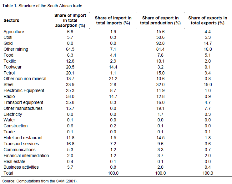
Our paper deals with the impact on trade liberalisation on the education sector, and specifically on students’ behaviour given fiscal constraints. From the Social Accounting Matrix (SAM) we use in the model, we can illustrate the relations between South Africa and  the  rest of the world. Table 1 points out the penetration rate of imports as well as the export intensity. It gives as well export intensity in sectoral production, and the share of each sector in total exports. It is relevant to notice that the two thirds of “other mineral” supply are imported. Moreover, radio equipment and transports equipment also strongly depend on imports. Given this structure, one can think that an increase in imports due to a decrease of tariffs will have strong consequences in these sectors. However, the three main sectors in total imports are the sector of other non-iron mineral products (Othnon, 21.2%): the Radio sector (14.7%) and the footwear sector (14.3%).

South Africa exports most of its production of mineral and precious metal, but we can also highlight its exports in hotel and restaurant sectors (14.5%), or in other industries (19.1%). Precious metal and mineral represent 65.2% of total exports of the country.

An external shock on mineral price would have strong effects on the economy. However, South Africa also exports  transports  services,  transports   equipment  and  other industries. As previously mentioned, South Africa has already cut its tariffs. However, for some commodities, tariffs remain quite high (for instance, footwear, other mineral and electronic equipment). These commodities will be sharply vulnerable to a tariff cut. Moreover, these sectors use a lot of intermediaries’ consumptions, meaning that a decrease in the production of these sectors will have consequences on other sectors, notably trade and petrol sectors. 

 

Our model is inspired by Decaluwé et al.’s (2001)^[1] model. We have changed several assumptions to better represent the South African economy. The labour force is disaggregated by population group and skill levels so that we end up with twelve different labour categories. Each activity uses capital and the different types of labour. We assume that there is unemployment on each labour market.

We have also disaggregated households such that we have households by population groups (African, Coloured, Indian and White). Then, we have specified households’ consumption with a Linear Expenditure System (LES) of Stone Geary (1954) function, and we assume that transfers between institutions are significant. Finally, we consider that South Africa cannot export as much as it wants by introducing an export demand function with determined elasticity.

We also assume that aggregate capital-skilled labour has a CES between capital and skilled labour, but is presumed to be very low (quasi-Leontief, at 0.1). This indicates that capital and skilled labour are complementary: some kinds of physical capital (such as a new type of electronic machinery) cannot be used to produce anything in the absence of skilled people.

In order to model students’ behaviour, we follow Lofgren and Diaz-Bonilla (2006). Students are classified into three educational sectors (primary, secondary and post-secondary). Each year, a student graduates (dip), drops out (aban) or repeats a grade (red).  Moreover, we assume that when a student graduates, she can go on studying (contdip) or enter the labour market (quitdip).

What determines the students’ behaviour?

We assume that a student’s decision is influenced by three variables:

(a) The quality of education, a variable which is directly linked to government spending. Indeed, if the government decides to increase the number of primary school teachers, we would expect improved quality due to a lower student to teacher ratio. Such an improvement in school quality would offer students more incentive to stay in school.  

(b) The wage differential between semi-skilled and low-skilled labour. If the average semi-skilled wage is sufficiently higher than the low-skilled one, the expectation of a higher income would act as an incentive for the student to continue their studies.

(c) The wage differential between semi-skilled and skilled labour. Continuing on to more advanced schooling would become more attractive if the average skilled wage is sufficiently higher than the semi-skilled one.  These changes in student’s behaviours have impacts on labour supply. Following Lofgren and Diaz-Bonilla (2006), we assume that for a given year, labour supply is equal to what it was the previous years plus the volume of students that enter the labour market depending on their success at school. We assume that students who graduate from their primary education level would enter the labour market as low skilled workers. Students who would graduate from the secondary education level would enter the labour market as a semi-skilled worker whereas a student that graduates from the tertiary education level would enter the labour market as a skilled worker. The students who do not manage to graduate and drop out would enter the labour market at the next lower level. Therefore, it is easy to understand the potential links between a given policy and the education sector: for instance, if skilled wage rate drops after a shock in the economy, students might be willing to enter the labour market as semi-skilled workers and they will not be keen in going on in the tertiary level. In the same way, a negative shock on public expenditure will probably affect the education quality, and therefore students’ behaviours.

To calibrate our model, we use the same Social Accounting Matrix as Cockburn et al. (2005). We used the same elasticity values as them for income and trade.

To calibrate unemployment rates, we use the Labor Force Survey (2001) and use a wage curve (Blanchflower and Oswald, 1995), given the elasticities computed by Kingdon and Knight (2006).

For the closure rules, the nominal exchange rate is fixed and is the numeraire of the model. As South Africa is a small country, world prices are fixed. The current account balance is exogenous. Labour supplies are fixed at the first period and then depend on students achievements. Capital demand is specific and exogenous at the first period, and then grows given the new investments made in the activity[2]

 

We analyse three scenarios of total tariff removal with different fiscal policies. In the  first  scenario, government does not offset the decrease in its tariffs income; in other words, government savings is endogenous and there is no fiscal policies set up. In the two other scenarios, we assume that government savings is fixed. To compensate the loss in its income tariffs, in the second scenario we assume that government sets up an indirect tax on products. In the third scenario, we assume that to keep its deficit constant, government reduces its public spending.

Impacts on government’s income and the relations with the rest of the world

The removal of tariffs leads, ceteris paribus, to two direct consequences:

On the one hand, receipts will decrease. This decrease in the receipts leads to a decrease in government’s income as well as a decrease in its savings if no mechanism is set up to balance the cut of duty receipts. That is what happens in the first scenario, government’s income decreases by -3.1% and its savings drop strongly (-16.6%). In the two other scenarios, by hypothesis, public deficit remains constant.

On the other hand, import prices are decreasing and this decrease will be stronger for former protected sectors. We expect that imports would increase, notably in footwear sector (+39.05%), in textile sector (+7.2%) and in electronic equipment (+4.6%). Moreover, the price of imports is decreasing, and this fall off will be greater for former protected sectors.

Former protected sectors will have to adjust to price decreasing, and so, they will have to decrease their price to remain competitive. Given that, we expect a decrease of production in some of these sectors, as well as a decrease of the working force. The decrease of the production in these sectors will decrease in the same proportion intermediate consumptions that will have a strong impact for trade sector.

The current account balance is fixed by hypothesis; the increase in imports must be joined to an increase of exports. We also assumed that South Africa cannot export as much as it wants, meaning that to export more, South Africa has to be more competitive. In other words, local producers have to decrease their prices.

Impacts on institutions’ income and total investment:

We saw that producers have to be  competitive to export more. Thus, whatever the scenario, it infers that the workforce decreases. It comes that wage rates are decreasing and unemployment rates are increasing.

Given the decrease in the wage rate, households’ income decrease as well as their savings, which is a proportion of their disposable income.

In the second scenario, we introduced an indirect tax on products. In other words, households do not really benefit from the decrease of import prices because they have to pay a new tax. In this scenario, the decrease of households’ consumption is greater than in the other.

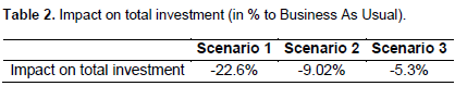
Firm’s income is mainly composed by capital income. We know that, given the numbers of firings, capital is relatively more abundant than labour. In the same way, the price decrease leads to a decrease of marginal productivity of capital; its return rate is decreasing. Thus, firm’s income is decreasing as well as its savings. Whatever the scenario analysed, total investment is decreasing (Table 2), and the decrease is stronger in the first scenario given the damage of public savings. 

 

 

Impact on the educational system

Previous effects are traditionally observed in short term for a trade liberalisation. Our aim is to analyse what happens on the education system, and notably if government has to reduce its spending in education to keep its deficit constant. Moreover, we know that trade liberalisation can have effects on wage rates, and these changes can have impacts on students’ behaviours. Indeed, as wage rate variations create incentives for students to go on studying or to enter the labour market, it is interesting to see how trade liberalisation affects students’ behaviours.

We saw that students’ behaviour is determined by the supply of education services (assumed constant in the two first scenarios), wage differential between skilled and semi-skilled, and wage differential between semi-skilled and unskilled. As education supply is assumed fixed in the two first scenarios, only these two variables can infer any changes on students’ behaviours.

Effects on education in these two scenarios are very low: given the decrease of the average wage rate, and the fact that the average skilled wage rate decreases more than the average semi-skilled wage rate, we can notice that the share of students that leaves secondary to enter the labour market is increasing slightly.

In the third scenario, we assume that government keeps its deficit  constant by decreasing its public spending. We know that public spending in education plays a key role in students’ behaviours. Thus, to balance a loss of duty receipts, government reduces its spending, that leads to a decrease of the quality of education in each sector (-2.77%). This decrease of the quality is followed by an increase of drop out and repetition rates and a decrease of graduation rate for each level of education. In the same way, the share of students that leave school after primary and enter the labour market is decreasing, whatever the population group (Table 3). 

 

 

In the short term, effects of full trade liberalisation are harmful for the South African economy as well as in the education sectors. If in the first scenario we observe a crowding-out effect, in the two other scenario, the layoffs lead to a decrease in wage rate and so a decrease in households income. Impacts on the education sectors are greater in the third scenario, given that the decrease in public spending is added to the changes in relative wages.

In the long run, for the first scenario, the loss in government’s income leads to an increase in its current deficit. This, as expected, has a negative impact on total investment. The drop in total investment affects most of the productive sectors that fire workers. Unemployment is going up while wage rate is going down. The drop in the wage rate, especially for skilled workers has an impact on students’ behaviour that does not continue after secondary education level.

In the second scenario, government’s savings is constant and the loss in tariff revenues is compensated by an increase in indirect taxes. This fiscal measure has quite a bad impact on the economy as it affects house-holds’ consumption and firms’ intermediate consumption. In other words, the benefits from trade liberalisation in terms of price decrease are lowered by the increase in the indirect tax. Here again, unemployment rates are increasing and we observe the same mechanism as in the first scenario for the impact on education.

It is actually in the third scenario that we observe huge impacts on education. Regarding the rest of the economy, we have the same effects as in the short run.

The education sector faces in the long run a sharp decrease of its resources, as government spending adjusts. It means that the number of teachers is decree-sing, or eventually schools are closing. This decrease in the supply of education services leads to a decline in the quality of the education system. Therefore, we observe that dropout rates and repetition rates are increasing, and graduation rate is therefore decreasing.

 

 

 

The aim of this paper is to analyze the impact of trade liberalisation on students’ behaviours. We evaluated this impact through two transmission channels, differential wage rates and public spending in education under three different fiscal scenarios. From our results, we find that setting up a full trade liberalisation without fiscal scenario is not sustainable in the long run, as the government’s deficit hampers total investment and GDP in the long run. The education sectors, and especially the post-secondary education sector, are affected through the decrease in skilled wages. Compensating the losses by increasing the indirect tax rate on commodities is as well harmful for the economy and the education sectors. From the last scenario, we can conclude that the variations of public spending have a stronger effect on students’ behaviours than wage rate changes. Then, given our results, we can say that a trade liberalisation policy that would lead government to decrease its public spending would have harmful consequences on education  sectors  as  well  as the whole economy.

However, we need to qualify our results as we simulated a full trade liberalisation in one shot. In this paper, we were more interested in understanding the mechanisms between trade liberalisation, different fiscal options and students’ behaviours.

The author has not declared any conflict of interests.