ABSTRACT
Knowledge of formation pore pressure ahead of the drill bit is not only critical for safe and cost-effective drilling of wells but also essential in studying the hydrocarbon trap seal and analyzing the trap configurations. A predrill estimate of the formation pore pressure can be obtained from seismic velocities and employing a velocity-to-effective stress transform. However, limitations abound in the use of seismic velocities for accurate pore pressure prediction. These limitations are traceable to some main factors such as the correctness of the seismic velocities themselves and the accuracy of the local parameters of the pore pressure prediction method used. Knowledge of the sources of overpressure in the formation is also an essential factor. This paper discusses these factors and attempts to put them into context for accurate pore pressure prediction using seismically-derived velocities.
Key words: Pore pressure prediction, overpressure, geopressure, seismic velocities, tomographic inversion, seismic inversion.
Knowledge of the formation of pore pressure before the drill bit has become even more critical as exploration and production (E and P) of oil and gas advance into more precarious environments. In the exploration stage, knowledge of the pore pressure will ensure better assessment of the trap integrity and basin geometry, as well as hydrocarbon migration pathways. In the drilling stage, accurate pore pressure prediction is important for safe and economic drilling.
Accurate poor pressure prediction is also essential for optimized casing program designed in order to avoid well control problems such as well kicks and blowouts, wellbore stability problems, stuck pipes, etc. Discussion on the subject of pore pressure has been receiving a great deal of attention for the last decades, especially in deepwater environments. Besides drilling a well, seismic survey is the only way to predict a potential geohazard subsurface zone apri-ori. Pioneering examples in the use of seismic data for geopressure prediction include the works of Hottman and Johnson (1965), Pennebaker (1968), Reynolds (1970, 1973).
Over the years, literature has been populated with works on the use of seismic data for predrill geopressure prediction. Of the various possible methods, the effective mstress method has become the preferred standard widely used in the industry, with the most popular method being the Eaton method (Eaton, 1975) and the Bowers method (Bowers, 1995). Even with the sophistication of parameters now in use and the range of software now available, limitations still abound in the use of seismic data for accurate pore pressure prediction.
These limitations can be traceable to the following main factors:
(1) Poor knowledge of the various sources of overpressure in the formation.
(2) The problem of accurate determination of the local parameters of the pore pressure prediction method used.
(3) Correctness of the seismic velocities themselves and the quality of the seismic data acquisition and processing technology.
This paper discusses these factors and highlights how they can be conditioned to ensure accurate pore pressure prediction using seismically-derived velocities.
The processes which generate overpressure in Tertiary basins where deposition and subsidence occur very rapidly can be categorized into three groups. The ability of each group to generate overpressure depends on the rock and fluid properties and their rate of change with the varying basin conditions.
Mechanisms related to increase in stress:
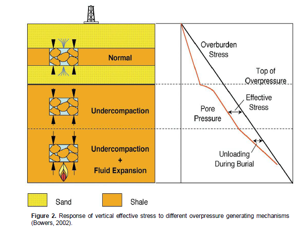
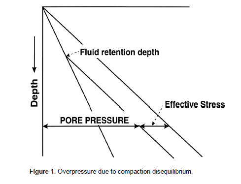
The primary source of overpressure in Tertiary basins is believed to be mechanical compaction disequilibrium in low permeability sediments. If the low permeability sediment does not allow the escape of the confined pore fluid at rates sufficient to keep with the rate of increase in vertical stress, in order to maintain a hydrostatic pressure gradient, the pore fluid is forced to carry a large part of the combined weight of the overlying rocks and fluids. This leads to increase in pore fluid pressure and results in under compaction or compaction disequilibrium in the rapidly accumulating sediment. This type of overpressure mechanisms is observed mainly in young tertiary basins worldwide and is commonly recognized in seismic velocity data by the slow decrease in velocity with depth.
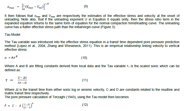
Overpressure due to compaction disequilibrium at a given depth is usually depicted by increase in porosity and typically occurs where there is a sand-rich to shale-rich environment. On pressure–depth plot (Figure 1), the mechanism is characterized by a fluid retention depth (FRD) at which overpressure starts and increases downwards along a gradient parallel to the lithostatic pressure gradient. This results in a constant vertical effective stress below the fluid retention depth and hence no further mechanical compaction or reduction in porosity takes place.
Another source of overpressure related to increase in stress is that related to tectonism (lateral compressive stress). This process is similar to undercompaction in that the increased vertical stress is taken up by the trapped pore fluid leading to an overall increase in geopressure (Dutta, 1987). However, unlike undercompaction, tectonic loading is capable of generating high overpressure (Bowers, 2002).
Mechanisms related to fluid volume expansion
A host of other overpressure generating mechanisms occur in addition to the primary undercompaction or compaction disequilibrium sources leading to the pore fluid volume expansion. These secondary mechanisms are usually due to in-situ fluid generating mechanisms which cause the pore pressure to increase at a fixed overburden, resulting in decrease of the effective stress on the matrix (Chopra and Huffman, 2006). Hence they are also known as unloading mechanisms. Some of the major mechanisms related to fluid volume expansion (Swarbrick and Osborne, 1998) include: aquathermal expansion, hydrocarbon source generation/maturation, clay diagenesis and oil to gas cracking.
Although the processes of overpressure generation in these mechanisms are distinctly different in their behaviour, they all produce similar effect in the rocks by resulting in the fluid volume expansion and the unloading mechanism of the formation for a given porosity. These overpressure mechanisms are commonly depicted by the reversal in the velocity trend with depth without an increase in porosity. Although not all velocity reversals are caused by overpressure, it is reasonable to treat velocity reversal as diagnostic feature of overpressure unless there is sufficient evidence from the well data to conclude that the velocity reversals are otherwise due to undercompaction, change in lithology or other possible causes. A deterministic indicator of high overpressure is when the sonic velocity and resistivity data have larger reversals than the bulk density data. This follows because transport properties such as sonic velocity, permeability and resistivity generally undergo more elastic rebound than bulk density and porosity (Bowers and Katsube, 2002).
Mechanisms related to fluid movement and buoyancy
These include other minor overpressure generating sources such as osmosis, hydrocarbon buoyancy, lateral transfer and hydraulic head (Swarbrick and Osborne, 1998). Figure 2 shows the pressure trend and response of vertical effect stress (VES) to different overpressure generating mechanisms.
PORE PRESSURE PREDICTION METHODS
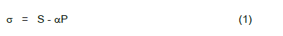
Most methods of pore pressure predictions are based on Terzaghi’s effective stress relation (Terzaghi, 1943) that expresses elastic wave velocity as a function of vertical effective stress. Since the stress is normal, it can otherwise be called pressure and be used interchangeably. The effective pressure, s, is the pressure acting on the solid rock matrix. It is defined as the difference between the overburden pressure, S, and the pore pressure, P. Terzaghi’s relation extended to solid rocks can be written as:
Where a is the poro-elastic coefficient, and is the ratio of the effect of fluid pressure on VES with the effect of overburden stress on VES. The poro-elastic coefficient is introduced in Terzaghi’s original equation when applied to consolidated rocks to take care of the effect of decrease in fluid pressure now applied on less of the grain surface. Generally, a < 1 and has a valve between 0.7 and 1.0; for over pressured rocks, a is usually around 0.8.
The overburden pressure is the pressure due to the combined weight of the rock matrix and the fluids in the pore space overlying the formation of interest at a given depth. The overburden pressure S can be expressed as integral of density:
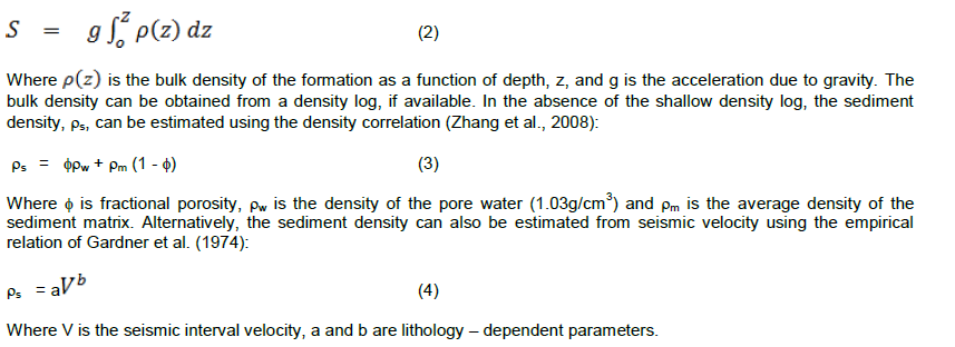
The compaction process of sedimentary rocks is essentially controlled by the effective stress. Hence any condition at a given depth that brings about a decrease in effective stress will ultimately lead to a decrease in the compaction rate (higher porosity) and consequently result in overpressure. Low effective stress and high porosity tend to lower the rock velocity. Thus, in young Tertiary basins such as the Niger, Nile and Mississippi deltas, Gulf of Mexico and Baran basins with thick intervals of shale and high sedimentation rate, it is geologically reasonable to use velocity as proxy for porosity retention to predict overpressure. Relationships between the rock velocity and the effective stress, and pore pressure, abound in literature (Hottman and Johnson, 1965; Mathew and Kelly, 1967; Eaton, 1972, 1975; Bowers, 1995; 2001; Flemmings et al., 2002).
If the relation between elastic wave velocity and vertical effective stress is known, the pore pressure P can be calculated from Equation 1, and the total overburden stress determined from Equation 2. Most common methods used for determining pore pressure from compressional seismic velocity include the Eaton’s method, Bowers’ method and the Tau model. The choice for each method depends on the overpressure generation mechanism in the area of interest.
Eaton’s method
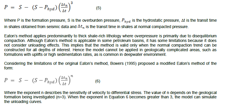
Eaton (1975) in accordance with Terzaghi (1943) presented an empirical relation for the pressure from compression transit time:
Bowers’ method
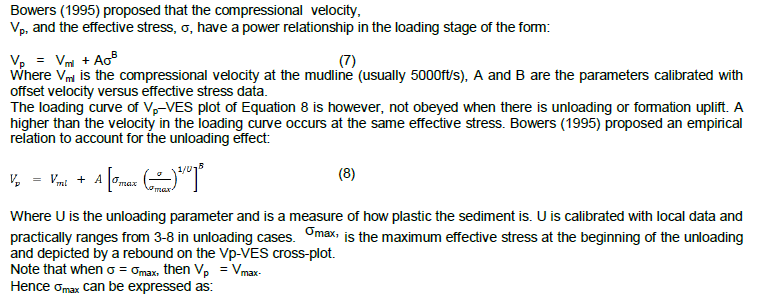
The power law nature of Equation 10 is theoretically sound and in practice has been widely proven to give more robust and excellent fit (Opara et al., 2013). It should be noted that the pore pressure prediction methods described in this paper are all based on the rock properties in shales. Hence the pore pressures obtained from these methods are the pressures in shales. For the pressures in sand, sandstones or other permeable formations, the formation pore pressure can be obtained by assuming that the shale pressure is equal to the sandstone pressure or using fluid flow model (Traugott, 1997; Zhang, 2011) to calculate the pressure.
SEISMIC VELOCITIES FOR PORE PRESSURE PREDICTION
The accuracy of predrill pore pressure prediction largely depends on the type of seismic velocity used for the velocity-pressure transformation and the quality of the data conditioning. Many types of seismic velocity analysis exist but for well planning purposes, the seismic velocities should be derived using methods that give sufficient spatial resolutions.
In the presence of complex or steeply dipping structures, the resolutions obtained from the conventional stacking velocity analysis are usually too low for accurate pore pressure prediction due to the layered earth model and hyperbolic move out assumptions. High resolution velocity analyses that have been used with varying degrees of success include the horizon-keyed velocity analysis, reflection tomography and seismic inversions. These techniques yield more robust geopressure predictions, though at higher cost. The resolution and accuracy of each technique depends, to a large extent, on the geologic scenario that plays out and on the expertise of the pressure interpreter.
Horizon – keyed velocity analysis
The horizon–keyed velocity analysis (HVA) provides accurate velocities at every CMP location along selected key horizons, as opposed to the conventional velocity analysis that is usually carried out at selected CMP locations. HVA is usually carried out using a small number of time gates centered on normal incidence travel times that track the given reflection horizons. The technique has been proven to be an efficient velocity analysis for geopressure prediction (Yilmaz, 1987).
Reflection tomography
In contrast to interval velocities resulting from conventional velocity analysis, reflection tomography (Stork, 1992; Woodward et al., 1998; Bishop et al., 1985), provides more detailed interval velocities necessary for predrill pore pressure prediction in terms of the spatial resolution. The velocity field resulting from reflection tomography better relates to the 3D geologic structures than that realizable with conventional stacking velocity analysis.
Reflection tomography is basically a 3D traveltime inversion process. The input to the process consists of travel time picks of the seismic reflection events and a first-guess velocity of the subsurface structure which characterizes the model. This is usually done in the depth domain rather than the time domain. Following the picking of the travel times from the seismic data and the computation of the travel times by ray tracing (Aki and Richards, 1980), the difference (misfit) between the two travel times is used to solve the least-squares equation of the form:
?T = D. ?S (13)
Where ?T is the difference between the real travel time picked from the seismic data and that estimated by ray tracing through the model. D is an nxm matrix containing the ray distances, n is the number of ray paths and m is the number of slowness cells.
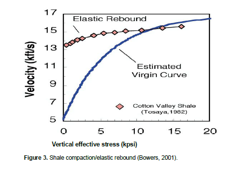
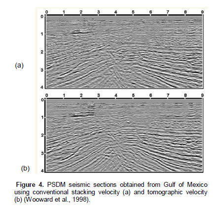
The least–squares slowness solution obtained is used to refine and update the original slowness model. The process is iterated until variations in ?S become insignificantly small. When properly conditioned, the tomography inversion velocity can provide a reliable velocity field which can closely relate to the rock velocity of the subsurface structure. Figure 4 shows the PSDM seismic sections from the Gulf of Mexico obtained by Woodward et al. (1998) using velocities derived by conventional stacking velocity (a) and velocity field refined by reflection tomography (b). Significant improvement in the seismic image is obtained with the velocity field refined by reflection tomography compared to that obtained by conventional stacking velocity field.
Sayers et al. (2002) demonstrates the pore pressure predictions arising from the two velocity fields (Figure 5). Although the velocity obtained from the stacking velocity analysis predicts the presence of overpressure in this area, the pore pressure prediction from the tomographically refined velocity model is more dramatic in terms of the magnitude and spatial resolution. Thus, robust pore pressure prediction requires very accurate velocity field with high spatial resolution akin to the tomographically refined velocity model.
Seismic inversion velocities
Seismic inversion generally refers to transformation of seismic amplitudes (prestack or postack) into acoustic impedance values. It is an integration of data from several sources, seismic, well log and/or velocity. Hence a good quality impedance model contains more information than the seismic reflection data. Acoustic impedance (product of velocity and rock density) being a layer property, and not an interface property, allows direct interpretation of 3D geologic structures.
For pore pressure prediction, seismic inversion can be carried out as a means of refining the velocity field in order to improve the resolution, and as a means of removing unwanted data from the pressure calculation. Usually, the inversion technique begins with a reliable velocity field. The velocity field is then refined and updated by the process.
Prestack inversion
Prestack seismic amplitude inversion methodologies are wave-equation–based. These full waveform techniques represent the generalized multidimensional inversion that allows the estimation of density and velocities (Vs and Vp) simultaneously, using the near offset reflectivity and amplitude versus offset behavior of each reflection event in the subsurface. This allows the user to estimate the overburden and effective stress from the same data set. They generally use seismic gathers as seed to produce the velocity model. The method employs inversion schemes based on nonlinear least–squares and updates the earth parameters iteratively in order to monotonically minimize the misfit between the observed and the modeled data.
Mallick (1999) developed a generic algorithm (GA) for prestack inversion which can be used to obtain the P-wave and the S-ware velocity models, and densities for a given seismic gather by minimizing the mismatch between the observed angle gathers and their corresponding synthetic computations. The process is iterated until the fitness values in the synthetic models converge.
Figure 6 shows the result of the application of the generic algorithm approach by Dutta (2002) to the CMP gathers for the stacked data, and the corresponding synthetic stacks. The biggest challenges to prestack inversion in pore pressure prediction, other than cost, are its extreme sensitivity to data quality and the need to incorporate the low-frequency velocity trend in the analysis which has its own attendant problems.

Postack inversion
Postack amplitude inversion like the prestack inversion provides high resolution by inverting for impedance from the seismic reflection services represented by the geologic formations. Seismic wavelet side lobes are removed from the reflection events to obtain estimates of residual impedance for each layer/lithology. The inversion can be used to generate estimates of the absolute impedance (Ip and Is) or its components of velocity and density (Vp, Vs, r).
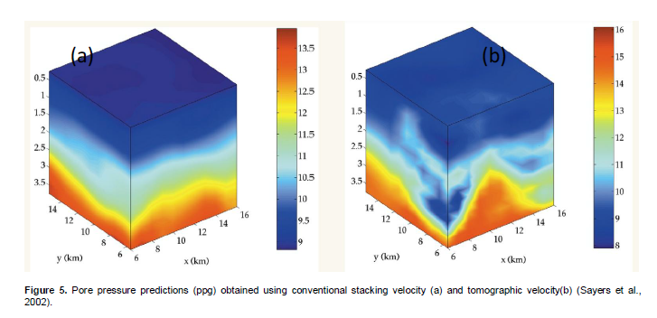
Postack inversion can be applied using only the stacked seismic data or can be calibrated with well logs, check shot or VSP data. Figure 7 shows the difference in resolution between conventional horizon–keyed velocity analysis and postack inversion presented by Huffman (2002). The postack inversion results show higher resolutions of the seismic traces.
Pore pressure prediction is key to safe and economic drilling. Pore pressure prediction from seismic survey uses seismically derived velocities to estimate the formation pore pressure. However, limitations abound in the use of seismic data for accurate pore pressure prediction, especially in precarious complex/steeply dipping structures or deepwater environment. Although there are different methods of estimating formation pore pressure, the applicability and accuracy of each method depends on accurate determination of the local parameters of the pore pressure prediction method used, the formation geology, the correctness of the seismic velocities and quality of the seismic data acquisition and conditioning.
The pressure interpreter should have a good understanding of the overpressure sources in the formation to be able to relate the pressure trend and response of vertical effective stress to the different overpressure generating mechanisms. Pore pressure prediction using seismic data requires seismic velocities that are dense and accurate and are close to the formation velocities under consideration. Such velocities with high resolutions akin to the tomographically refined velocities and inversion velocities yield robust geopressure predictions, though at higher cost.
REFERENCES
Bishop TN, Bube KP, Cutlers RT, Langan RT, Love PL, Resnick JR, Shuey RT, Spindler DA, Wyld HW (1985). Tomographic determination of velocity and depth in laterally varying media, Geophysics, 50:903-923.
Crossref |
|
|
|
Bowers GL (1995). Pore pressure estimation from velocity data: accounting for overpressure mechanisms besides undercompaction, SPE Drilling and completions. |
|
|
|
Bowers GL (2001). Determining an appropriate pore pressure estimation strategy, Offshore Technology Conference, Paper OTC 13042. |
|
|
|
Bowers GL (2002). Detecting high overpressure, The Leading Edge, SEG Publication, pp. 174-177. |
|
|
|
Bowers GL, Katsube IJ (2002). The role of shale pore structure on the sensitivity of wire line logs to overpressure, in Huffman AR and Bowers GL (eds), Pressure Regime in Sedimentary Basins and their Prediction, AAPG, Memoir P. 76. |
|
|
Chopra S, Huffman AR (2006). Velocity determination for pore pressure prediction, The Leading Edge, 23(12):1502-1515.
Crossref |
|
|
|
Dutta NC (Editor) (1987). Geopressure, Geophysics Reprint Series No. 7, Society of Exploration Geophysicists. |
|
|
Dutta N (2002). Geopressure prediction using seismic data: Current status and the road ahead, Geophysics, 67(6):2012-2041.
Crossref |
|
|
|
Eaton BA (1972). Graphical method predicts geopressure worldwide, World Oil, 182:51-56. |
|
|
|
Eaton BA (1975). The equation for geopressure prediction from well logs, Soc. Petr. Engineers, Paper SPE 5544. |
|
|
Flemmings PB, Stump BB, Finkbeiner T, Zoback M (2002). Flow focusing in overpressured sandstones: theory, observations and applications. Am. J. Sci. 302:827–855.
Crossref |
|
|
Gardner GHF, Gardner LW, Gregory AR (1974). Formation velocity and density – the diagnostic basis for stratigraphic traps. Geophysics, 39(6):2085–2095.
Crossref |
|
|
Hottman CE, Johnson RK (1965). Estimation of formation pressures from log derived shale properties, J. Pet. Technol. 6:717-722.
Crossref |
|
|
Huffman AR (2002). The future of pore pressure prediction using geophysical methods, in Huffman AR and Bowers GL (eds.), Pressure regimes in sedimentary basins and their predictions, AAPG Memoir 76:217-233.
Crossref |
|
|
Lopez JI, Rappold DM, Ugueto GA, Wieseneck JU, Vu K (2004). Integrated shared earth model: 3D pore pressure prediction and uncertainty analysis, The Leading Edge, pp. 152-159.
Crossref |
|
|
|
Mathew WR, Kelly J (1967). How to predict formation pressure and fracture gradient: Oil Gas J. pp. 92-106. |
|
|
Mallick S (1999). Some practical aspects of prestack waveform inversion using a generic algorithm: An example from East Texas Woodbine Gas Sand, Geophysics 64(2):326-336.
Crossref |
|
|
|
Opara AI, Onuoha KM, Anowai C, Onu NN, Mbah RO (2013). Geopressure and trap integrity predictions from 3-D seismic data: case study of the Greater Ughelli Depobeit, Niger Delta. Oil and Gas Science and Technology – Rev. IFP Energies nouvelles, 68(2):383-396. |
|
|
|
Pennebaker ES (1968). Seismic data indicate depth and magnitude of abnormal pressure, World Oil, 166:73-82. |
|
|
|
Reynolds EB (1970). Predicting overpressured zones with seismic data; World Oil 171:78-82. |
|
|
|
Reynolds EB (1973). The application of seismic techniques to drilling techniques, Soc. Petr. Engineers, Preprint 4643. |
|
|
Sayers CM, Woodward MJ, Bartman RC (2002). Seismic pore-pressure prediction using reflection temography and 4-C seismic data, The Leading Edge 21(2):188-192.
Crossref |
|
|
Stork C (1992). Reflection tomography in the post migrated domain. Geophysics 57(5):680-692.
Crossref |
|
|
|
Swarbrick R, Osborne MJ (1998). Mechanisms that generate abnormal pressures: An overview, in Law BE, Ulmishek GF, Slavin VI (eds), Abnormal pressures in hydrocarbon environments, AAPG Memoir 70:13-34. |
|
|
Terzaghi K (1943). Theoretical soil mechanics, John Wiley and Sons, Inc.
Crossref |
|
|
|
Traugott M (1997). Pore and fracture pressure determination in deepwater. World Oil 218(8):68-70. |
|
|
|
Woodward M, Farmer P, Nickolas D, Charles S (1998). Automated 3D tomographic velocity analysis of residual moveout in prestack depth migrated common image point gathers, Expanded Abstracts, 68th Intl. Ann. Meeting, SEG, pp. 1218-1221. |
|
|
Zhang J (2011). Pore pressure prediction from well logs, modifications and new approaches. Earth Sci. Rev. 108:50-63.
Crossref |
|
|
Zhang J, Wieseneck J (2011). Challenges and Surprises of Abnormal Pore Pressure in the Shale Gas Formations. SPE Annual Technical Conference and Exhibitions. Paper SPE 145964.
Crossref |