ABSTRACT
Information about data arrangement methodologies and optimal sample size in estimating the Pearson correlation coefficient (r) among maize traits are still limited. Furthermore, some data arrangement methodologies currently used may be increasing multicollinearity in multiple regression analysis. This study aimed to investigate the statistical behavior of the r and the multicollinearity of correlation matrices among maize traits in different data arrangement scenarios and different sample sizes. Data from 45 treatments [15 simple maize hybrids (Zea mays L.) conducted in three locations] were used. Eleven traits were accessed and three datasets (scenarios) were formed: (1) Coming from all the sampled observations (plants), n = 900; (2) Coming from the average of five plants per plot, n = 180; and (3) Coming from the average of treatments, n = 45. A thousand estimates of r were held in each scenario to 60 sample sizes by bootstrap simulations with replacement. Confidence intervals (CI) were estimated. One hundred eighty correlation matrices were estimated and the condition number (CN) calculated. Data coming from average values of plots and average values of treatments overestimates the r up to 24 and 34%, resulting in an increase of 24 and 131% in the matrices’ CN. Trait pairs with high r require a smaller number of plants, being the CI inversely proportional to the magnitude of the r. Two hundred and ten plants are sufficient to estimate the r in the CI of 95% < 0.30.
Key words: Average values, bootstrap, confidence intervals, sample tracking, Zea mays L.
Abbreviation:
ASO, all sampled observations; AVP, average values of plot; AVT, average values of treatments; CD, cob diameter; CD/ED, cob diameter/ear diameter ratio; CL, cob length; ED, ear diameter; EH, ear height; EL, ear length; NKR, number of kernels per row; NRE, number of rows per ear; PH, plant height; TKW, thousand-kernel weight; TNK, total number of kernels per ear.
One of the most used statistical methods to measure the degree of association (linear) between two random traits is the Pearson product-moment correlation coefficient (r) (Pearson, 1920) and has been used in ecological studies to estimate the direction and degree of association among traits (Annicchiarico et al., 1999; Yao and Mehlenbacher, 2000; Yang and Su, 2016).
As this measure only reveals the linear association between two traits, techniques such as path analysis (Wright, 1923) and canonical correlation (Hotelling, 1936) were developed in order to explain the interrelationships among traits or group of traits, being worldwide used in plant breeding. These techniques depend on the linear correlation matrix among traits and, due its estimates be based on principles of multiple regression, the low dependence among the traits considered as explanatory is required. When this assumption is not met, it is said that the matrix presents multicollinearity (Blalock, 1963).
Although there are techniques to adjust the multicollinearity (Hoerl and Kennard, 1970b) these techniques are essentially correctives, applied only after the linear correlation matrix be estimated. Since the estimates of correlation coefficients basically involve the behavior analyses of the variances, that is, deviations from the average, it is possible that some methods of data arrangement currently used may be masking the actual averages and variances of a trait (X) on a dataset of (n) observations. For example, in a bibliographic survey, we found that the correlation matrices of some agronomic studies using path analysis were estimated with average values of several plants sampled in each experimental unit (Khameneh et al., 2012; Toebe and Cargnelutti 2013; Adesoji et al., 2015; Kumar and Babu, 2015; Nataraj et al., 2015).
In field experiments, it is very common to access values of traits in several plants of each experimental unit. The utilization of average value of these plants in order to estimate the r and perform inferences to the population under study, however, may be questionable. In a theoretical explanation focused on plant breeding, Olivoto et al. (2016) reported that the use of average values in estimating the r between a traits pair (e.g. rx:y) may overestimate its magnitude mainly due the reduction of standard deviation (SD) in the dataset, when compared with estimates performed with values coming from all sampled plants. In addition, the observed SD (e.g. for X and Y) when average values of plots or treatments are used, represents the SD of the average of the originally sampled plants, and not the actual SD coming from all these plants; therefore, this SD is masked and tends to present lower itself. This fact should be taken into consideration, because the inference of the direction and magnitude of association among traits when average values are used is being made for a different population of the original.
There were no studies in the literature comparing different data arrangement methodologies on estimates of Pearson’s correlation coefficients. In addition, the information about the optimal sample size in order to estimate the r among trait pairs in the maize crop in an acceptable confidence interval is needed. In this context, the aims of the present study were to (i) reveal the statistical behavior of estimated Pearson’s correlation coefficients in different data arrangement scenarios and different sample sizes, (ii) reveal the impact of data arrangement scenarios and sample sizes on multicollinearity of matrices, and (iii) propose the optimal sample size in order to estimate r among trait pairs in the maize crop in an acceptable confidence interval.
Site description and experimental design
Field trials were conducted in 2014/2015 growing season in Santo Expedito do Sul (27°56' S, 51°37' W; 728 m asl), São José do Ouro (27°44' S, 51°32' W; 796 m asl) and Viadutos (27°33' S, 52°00' W; 628 m asl), municipalities of Northeastern Rio Grande do Sul State, Brazil. During the experimental period, the air averages temperatures at the sites of the experiments were 24.5, 23.8 and 25.2ºC and the natural rainfall of 823, 958 and 746 mm, respectively. All locations are within a 70-km radius, have a Haplustox soil, and were chosen due to similarities of soil and climatic characteristics, which provided to them low variability of temperature and rainfall. Thus, abiotic effects on the plants’ response were minimized as much as possible.
Prior to the installation of the trials, each site was surveyed for potentially disruptive characteristics. To ensure uniformity inside the block and heterogeneity between the blocks, a randomized complete block design in a 15 × 3 factorial treatment design (15 simple maize hybrids x three cropping fields) with four replications was used, totaling 180 plots. Each plot contained six 5-m-long cultivar rows, spaced by 0.45 m. Only the two central rows were used to prevent edge effects. In each plot, five representative plants (observations) were selected from which the ear was removed for further evaluation. To ensure that traits (of plant and ear) were assessed in the same individual, a sample tracking system was created, identifying each ear with a label containing a sequence number that characterized the site, the hybrid, the repetition and the evaluated plant.
Accessed traits
Plant height (PH) and the ear insertion height (EH) were measured (cm) from the ground surface to the flag leaf node and the support node of the highest ear at the stem, respectively. Tagged ears were evaluated at a laboratory. The following traits were accessed: ear length (EL) (cm), ear diameter (ED) (cm), number of rows per ear (NRE) (un), number of kernels per row (NKR) (un), cob length (CL) (cm), cob diameter (CD) (mm), cob diameter / ear diameter ratio (CD / ED) (decimal), total number of kernels per ear (TNK) (un) the thousand-kernel weight (TKW) (g). The ratings were performed as follows: The lengths and diameters were measured with a digital caliper. After counting the number of rows per ear and the number of kernels per row, the kernels of each ear were manually-threshed and cleaned with pressurized air. Subsequently, the kernels-weight was measured with an analytical balance and the total number of kernel each ear was measured with seed counter equipment. Finally, the grain moisture was measured with a universal moisture meter. With this data, and with the humidity adjusted to 14% base moisture, we determined the thousand-kernel weight each ear by the equation: TKW = [(KME/TNK) × 1000]. Where: TKW = Thousand kernel weight; KME = Kernel mass per ear; TNK = the total number of kernels per ear. All evaluations were carried out carefully in an ear at a time, to maintain traceability of the sample, avoid any systematic errors as well as minimize the random errors.
Statistical procedures
Bootstrap simulations
Three data arrangement scenarios were considered: (i) The data used were originated from all sampled observations (ASO), with a total sample size of 900; (ii) In this scenario, the data used were obtained from the average of the five sampled plants of each plot (AVP), with a total sample size of 180, and (iii) Finally, the average of the treatments (15 treatments × 3 locations), with a total sample size of 45 was considered (AVT).
Aiming to match the sample size in each scenario, 60 sample sizes (plants) were simulated. The size of the initial sample was 15 plants, and the rest were obtained with an increment of 15 plants up to 900 plants. For each one of 55 trait pairs [n × (n-1)]/2, where n =11, in each sample size of each scenario, 1000 simulations of the r were performed by bootstrap resampling with replacement (Efron, 1979). Thus, for each pair of traits, 1000 estimates of the r were obtained. Simulations were performed by the Structural Equation Modeling procedure in Statistica 10.0 software.
Descriptive analysis of correlation coefficients
In each sample size of each scenario, the 1000 simulated r were subjected to descriptive analysis, where it was determined the maximum, (97.5%), average, (2.5%) and minimum values. Later, the amplitude of the 95% confidence interval was calculated by the difference between the percentile 97.5 and 2.5%. For comparison, three trait pairs that came closest to the following r magnitudes were chosen: r ≈ |0|, r ≈ |0.5| and r ≈ |1.0|. The statistics mentioned of these three trait pairs has formed scatter diagrams where the x-axis corresponds to the number of plants and the y-axis corresponding to the descriptive statistics.
t-test to compare the correlation coefficient among the scenarios
In order to determine whether the inferences could be made with the average of 60 sample sizes, initially the r average of each traits pair at the different sample sizes were compared by t-test at 5% probability error (Steel et al., 1997) in the following scenario combinations: ASO × AVT, ASO × AVP and AVP × AVT. Inferences were made using the average of sample sizes for each pair of traits if the 60 samples presented the same result on the test.
A test comparing the 3300 values of r (55 trait pairs × 60 sample size) was also performed. Histograms were developed for each scenario combination (ASO × AVT, ASO × AVP and AVP × AVT) in order to show the behavior of the estimated r distribution. These procedures were performed using t.test and hist functions in R software (R core Team, 2016). Descriptive statistics such as asymmetry, average, mode, 25th and 75th percentiles, maximum, and minimum applied in each scenario are also presented in boxplot graphics. These procedures were performed using summary and boxplot functions in R software.
Diagnosis of multicollinearity in the scenarios
Data of 11 traits obtained by the average of 1000 bootstrap simulations in each sample size of each scenario were used in order to estimate correlation matrices. A total of 180 matrices (60 sample size x three scenarios) were estimated. In each matrix, multicollinearity diagnosis was performed by the condition number (CN) of the matrix. The CN was obtained by the ratio between the largest and the smallest eigenvalue of the matrix. The degree of multicollinearity was considered weak, moderate and severe when CN ≤ 100, between 100 and 1000 and ≥ 1000, respectively (Mansfield and Helms, 1982). A graph containing the number of plants (x-axis) and the CN of each scenario (y-axis) was developed. This analysis was performed using the Multicollinearity Diagnostic procedure in Genes software (Cruz, 2013).
Statistical properties of the correlation coefficient
The estimated r presented the largest amplitude when the lowest number of plants was used. For the pair EH x PH, the magnitude of r oscillates between -0.02 and 0.98 (Figure 1a), 0.42 to 0.99 (Figure 1b) and 0.71 to 0.99 (Figure 1c) in ASO, AVP, and AVT scenarios, respectively. This range was reduced as the number of plants increased; however, it appeared higher in the ASO scenario. The average r between the 60 different numbers of plants evaluated was increased by approximately 11% (r = 0.92) and 15% (r = 0.96), in AVP and AVT scenarios, respectively (Figure 1b and c).
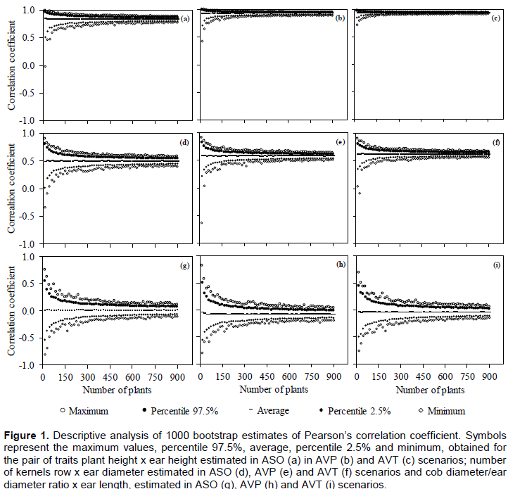
For trait pairs with r ≈ | 0.5 | as NKR × ED, the amplitude of r was larger, irrespectively of the scenario and the number of assessed plants. With 15 plants, r ranged between -0.33 and 0.89 in the ASO scenario (Figure 1d), between -0.62 and 0.91 in the AVP scenario (Figure 1e) and between 0.03 and 0.90 in the AVT scenario (Figure 1f). The average r was increased by approximately 16% (r = 0.58) and 24% (r = 0.62), in AVP and AVT scenarios, respectively. Trait pairs with r ≈ | 0 | as DSDE x CE presented the highest amplitudes, with similar r distribution in the studied scenarios (Figure 1g to i).
For the pair PH × EH, 270 plants were enough to estimate the r in the ASO scenario in the CI 95% ≤ 0.10 (Figure 2a). For AVP and AVT scenarios, however, the number of plants needed was only 45 (Figure 2b) and 30 (Figure 2c), respectively. Trait pairs with r ≈ | 0.5 | (NKR x ED), needed 660, 465 and 285 plants, in ASO, AVP, and AVT scenarios, respectively. For CD/ED x EL combination, CI 95% ≤ 0.10 was not reached even with 900 plants.
Comparison of correlation pairs between the scenarios
The t-test revealed no differences among the sample sizes in all scenario combinations. Thus, the inferences for each pair of traits were performed with the average of 60 sample sizes. Among the 165 comparisons (55 trait pairs in three scenario combinations), 164 differed. Only one did not differ. In approximately 82% of the cases, average values (AVT and AVT scenarios) overestimated the magnitude of the r (Table 1).
Comparing the estimated r in ASO × AVT scenarios, of 55 tested pairs, ten (18%) had a higher average when all sampled observations were used (Table 1). Comparing ASO × AVP scenarios, only seven combinations (13%) had a higher average r in correlation analysis estimated with all observations. Comparing the averages (AVP × AVT), 12 combinations (22%) were higher when the average of the plots was used (Table 1).
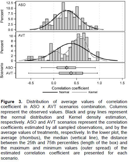
A t-test comparing the average r of 55 trait pairs in ASO x AVT scenario combination confirmed the difference between these (t-value = -12.89, P < 0.001). The average r with low magnitudes is due to the use of all pairs of correlation, where there are positive and negative values. The estimates in the ASO scenario showed a distribution similar to normal. That is related to the low asymmetry value (0.009), smaller r amplitude (-0.273 to 0.912), and the median value (0.268) that is similar to the average value (0.282), although the tests reject the hypothesis of normality (Kolmogorov-Smirnov = 0.048, P < 0.01) (Figure 3). The estimates carried out in the AVT scenario, however, shows a negative asymmetrical distribution of r values (-0.843), with a greater r amplitude (-0.552 to 0.956) and the median value (0.484), higher than the average (0.379). The distribution of r values in this scenario do not follow the normal distribution (Kolmogorov-Smirnov = 0.137, P = < 0.01) (Figure 3).
The comparison of ASO × AVP scenarios shows a behavior similar to that discussed previously, though with a slightly smaller difference (t-value = -9.60, P < 0.0001). For the AVP scenario, r also presented negative asymmetry (-0.566). The amplitude was also lower (-0.427 to 0.926), with a median value (0.399) higher than the average (0.350) (Figure 4). The distribution in this scenario was not normal (Kolmogorov-Smirnov = 0.136, P < 0.01).
The t-test comparing the average r between the AVP × AVT scenarios combinations, revealed difference (t-value = -3.73, P < 0.001). With the measures of central tendency and amplitudes of these scenarios discussed above, both showed a non-normal distribution of r, with a clear tendency of most of the observed values being higher than r average (Figure 5).
The r was increased by approximately 24 and 34% in the AVP and AVT scenarios, respectively. In addition, the r amplitude and standard deviation were higher in these scenarios (Figure 6).
Multicollinearity
Multicollinearity was considered severe for the three scenarios, regardless of the number of assessed plants (Figure 7). The use of averages (AVP and AVT scenarios) increased the CN of the correlation matrices. The largest changes occurred when the number of plants was low (n < 100). For example, with 45 and 60 plants, the CN increased by 118 and 75% for the AVP scenarios and 250 and 68% for the AVT scenario, respectively. Although in some cases the CN was higher for the ASO scenario, on mean, CN was increased by 24 and 131% in AVP and AVT scenarios, respectively (Figure 7).
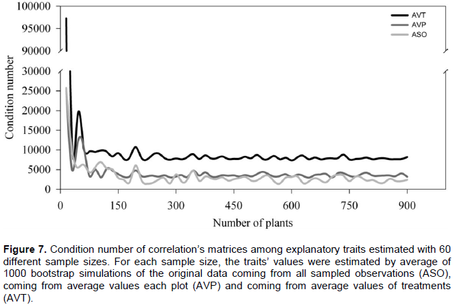
Average values represent 1000 bootstrap simulations of the original data coming from all sampled observations (ASO), coming from the average of each plot (AVP) and coming from the average of treatments (AVT). Coefficients in bold indicate the pairs in which r was lower with the use of averages. ‘*’ and ‘**’ show the significances at 0.001 and 0.01 of probability level, respectively. ‘ns’ is not significant. PH, Plant heigth; EH, ear heigth; EL, ear length; ED, ear diameter; NRE, number of rows per ear; NKR, number of kernels per row; CL, cob length; CD, cob diameter; CD/ED, cob diameter / ear diameter ratio; TNK, total number of kernels per ear; TKW, thousand-kernel weight.
The reduction of individual variation (standard deviation) observed in the scenarios AVP and AVT was the main factor responsible for overvaluing the r of trait pairs. This fact can be explaining due standard deviation be the divisor on correlation’s formula. If covariance XY (dividend of formula) is similar in both scenarios, however, the standard deviation of X and Y traits (divisor of formula) are smallest, the magnitude of correlation coefficients will be greater.
The higher number of plants required for estimation of the r at the 95% CI ≤ 0.10 in trait pairs with less intensity of linear association, shows that the researcher must take into consideration the magnitude of the trait pairs, being that the confidence interval will be inversely proportional to the magnitude of its correlations. The magnitude of the CI used here (95% CI ≤ 0.10) it is not a rule, being that each researcher must adopt the appropriate confidence level for its inferences. If we consider the CI 95% CI < 0.30, 210 plants are enough for estimating trait pairs with low magnitude (r < 0.10). This number of plants it is perfectly possible of to be evaluated. The experimental design (number of treatments and repetitions) will set then, the number of plants to be sampled in each plot. In experiments with large numbers of experimental units (e.g. factorial designs), the increase in sample size will provide greater confidence in the estimates provided that they are properly followed the sampling procedures and maintained traceability of these samples.
Although for trait pairs with high linear association (EH x PH) AVP and AVT scenarios needed 83 and 89% fewer plants to estimate r, the average r in these scenarios was increased by 11 and 15%, respectively, compared to the ASO scenario (r = 0.83). In an analysis that depends on of the linear correlation matrix for their estimates, e.g., canonical correlation, path analysis and stepwise multiple linear regression procedures, high linear association magnitudes among explanatory traits make it difficult to analyze, threatening the statistic and the inferential interpretation (Graham, 2003).
A recent study revealed that multicollinearity begins to seriously distort the estimates of the path coefficients when the explanatory traits show r > | 0.7 | (Dormann et al., 2013). While there have been observed high correlations in the ASO scenario (e.g. EH x PH, r = 0.83), the higher values for the same pair (r = 0.92) and (r = 0.96) estimated in APV and AVT scenarios, respectively, demonstrated that these data arrangement methodologies overestimate the magnitude of the r and may result in larger problems in estimates of multiple regression parameters, leading to an erroneous interpretation of predictors in a statistical model. Thus, these methods must be carefully evaluated by the researchers when the goal is to use the correlation matrix in studies involving multiple regression, as for this, the independence or the less degree of dependence among explanatory traits is sought (Prunier et al., 2014; Montgomery et al., 2012)
Average values (AVP and AVT scenarios), visibly elevated the multicollinearity of the matrices, confirming the earlier discussion. Although there are variations in CN in each studied sample size, the multicollinearity was increased on average by 24 and 131% when the AVP and AVT scenarios were considered in the estimation of correlation matrices. Although there are techniques for adjusting the multicollinearity as to delete the traits responsible for inflating the variance of the coefficients Gunst and Mason, 1977) or to perform estimates by using equations partially modified by the inclusion of a k constant in the diagonal elements of correlation matrix (Hoerl and Kennard, 1970a), these techniques can mask the true biological behavior’s response, because the deletion of the traits can reduce the model’s explanation power. The inclusion of the k constant is effective in reducing the magnitude of multicollinearity, however, also causes a bias in the regression analysis (Hoerl and Kennard, 1970a)
The best strategy to mitigate the problems caused by multicollinearity is to reduce it since it becomes practically impossible to eliminate it. In this research, a simple method for mitigating the multicollinearity in correlation matrices is suggested: estimating the correlation coefficients considering all observations, maintaining traceability and individual variance of the sample. This can be accomplished without significant increase of time, labor and financial resources since, a priori, all sampled plants were assessed.
Estimates made with data based on averages (AVP and AVT scenarios) reduce the individual variances, overestimate the correlation coefficients and increase the multicollinearity in correlation matrices. Thus, studies that require explanatory traits in order to predict a dependent trait will present greater misstatements in the estimates of the regression coefficients, if these methods are used. By using values coming from all sampled plants, 210 plants are enough for estimating Pearson product-moment correlation coefficients among maize traits in the bootstrap confidence interval of 95% < 0.30. The current study about data arrangement on Pearson’s correlation coefficients presents useful information on the planning of future experiments in plant breeding involving biometric templates that require the correlation matrix for their estimates.
The authors have not declared any conflict of interests.
REFERENCES
|
Adesoji AG, Abubakar IU, Labe DA (2015). Character association and path coefficient analysis of maize (Zea mays L). grown under incorporated legumes and nitrogen. J. Agron. 14(3):158-163.
Crossref
|
|
|
|
Annicchiarico P, Piano E, Rhodes I (1999). Heritability of and genetic correlations among, forage and seed yield traits in Ladino white clover. Plant Breed. 118(4):341-346.
Crossref
|
|
|
|
|
Blalock HM (1963). Correlated independent variables: the problem of multicollinearity. Social Forces 42(2):233-237.
Crossref
|
|
|
|
|
Cruz CD (2013). GENES: a software package for analysis in experimental statistics and quantitative genetics. Acta Sci. Agron. 35:271-276.
Crossref
|
|
|
|
|
Dormann CF, Elith J, Bacher S, Buchmann C, Carl G, Carré, G, Marquéz JRG, Gruber B, Lafourcade B, Leitão PJ, Münkemüller T, Mcclean C, Osborne PE, Reineking B, Schröder B, Skidmore AK, Zurell D, Lautenbach S (2013). Collinearity: a review of methods to deal with it and a simulation study evaluating their performance. Ecography 36(1):27-46.
Crossref
|
|
|
|
|
Efron B (1979). Bootstrap methods: another look at the jackknife. Ann. Statist. 7(1):1-26.
Crossref
|
|
|
|
|
Graham MH (2003). Confronting multicollinearity in ecological multiple regression. Ecology 84(11):2809-2815.
Crossref
|
|
|
|
|
Gunst RF, Mason RL (1977). Advantages of examining multicollinearities in regression analysis. Biometrics 33(1):249-260.
Crossref
|
|
|
|
|
Hoerl AE, Kennard RW (1970a). Ridge regression: biased estimation for nonorthogonal problems. Technometrics 12(1):55-67.
Crossref
|
|
|
|
|
Hoerl AE, Kennard RW (1970b). Ridge regression: applications to nonorthogonal problems. Technometrics 12(1):69-82.
Crossref
|
|
|
|
|
Hotelling H (1936). Relations between two sets of variates. Biometrika 28(3/4):321-377.
Crossref
|
|
|
|
|
Khameneh MM, Bahraminejad S, Sadeghi F, Honarmand SJ, Maniee M (2012). Path analysis and multivariate factorial analyses for determining interrelationships between grain yield and related characters in maize hybrids. Afr. J. Agric. Res. 7(48):6437-6446.
Crossref
|
|
|
|
|
Kumar SVV, Babu, DR (2015). Character association and path analysis of grain yield and yield components in maize (Zea Mays L). Electronic J. Plant Breed. 6(2):550-554.
|
|
|
|
|
Mansfield ER, Helms BP (1982): Detecting multicollinearity. Am. Stat. 36(3):158-160.
Crossref
|
|
|
|
|
Montgomery DC, Peck EA, Vining GG (2012). Introduction to linear regression analysis 5th ed John Wiley & Sons New Jersey.
|
|
|
|
|
Nataraj V, Shahi JP, Vandana D (2015). Character association and path analyses in maize (Zea mays L). Environ. Ecol. 33(1):78-81.
|
|
|
|
|
Olivoto T, Nardino M, Carvalho IRC, Follmann DN, Szareski VJ, Ferrari M, Pelegrin AJ, Souza VQ (2016). Pearson correlation coefficient and accuracy of path analysis used in maize breeding: a critical review. Int. J. Curr. Res. 8(9):37787-37795.
|
|
|
|
|
Pearson K (1920). Notes on the history of correlation. Biometrika 13(1):25-45.
Crossref
|
|
|
|
|
Prunier JG, Colyn M, Legendre X, Nimon KF, Flamand MC (2014). Multicollinearity in spatial genetics: separating the wheat from the chaff using commonality analyses. Mol. Ecol. 24(2):263-283.
Crossref
|
|
|
|
|
R core Team (2016). R: A language and environment for statistical computing. R Foundation for Statistical Computing, Vienna.
|
|
|
|
|
Steel RGD, Torrie JH, Dickey D (1997). Principles and procedures of statistics: a biometrical approach 3rd ed McGraw-Hill New York NY, USA.
|
|
|
|
|
Toebe M, Cargnelutti A (2013). Multicollinearity in path analysis of maize (Zea mays L). J. Cereal Sci. 57(3):453-462.
Crossref
|
|
|
|
|
Wright S (1923). The theory of path coefficients a reply to Niles's criticism. Genetics 8(3):239-255.
|
|
|
|
|
Yang H, Su G (2016). Impact of phenotypic information of previous generations and depth of pedigree on estimates of genetic parameters and breeding values. Livest. Sci. 187:61-67.
Crossref
|
|
|
|
|
Yao Q, Mehlenbacher SA (2000). Heritability, variance components and correlation of morphological and phenological traits in hazelnut. Plant Breed. 119(5):369-381.
Crossref
|
|