Mathematical models were developed, using 22 different genotypes of citrus, to estimate leaf area. The information of the relationship between leaf length and width (L/W)2 for simple leaf blade form (eliptic, ovate, obovate, lanceolate); and length of the three folioles (L2+L3)/L1 for a compound leaf (trifoliate leaves), was used with the purpose to separate group of similarities of leaf blade form and promote high accuracy of estimate. The best models presented an excellent precision with errors varying from 1.2 to 6.2 (%) and r2 higher than 0.95 for the majority of the models tested. Considering a single leaf blade, the linear model (Y = β . L . W) presented the lower mean deviation and lower square deviation. For the compound leaves, the potential models are simple to use, since use only the information of length of central foliole L1 (Y= β L1µ), although the use of linear models gave the best precision, as observed by using the model Y = β . L1 . W1. Furthermore the model might be used as a single model independent of the relation (L2+L3)/L1∶ {Y=β⋅(L1⋅W1 + L2⋅W2 + L3⋅W3), r² = 0.98}.
Leaf area is a variable of extreme importance to physiological and agronomic studies, such as vegetable growing, interception of light, remote sensing, photosynthetic efficiency, absorption of carbon, evapotranspiration, absorption of agrochemicals by the leaves, assessment of pest attack and irrigation management (Coelho Filho et al., 2004, 2012; Guimarães et al., 2013; Griffith et al., 2011; Lopes and Pinto, 2005; Oliveira et al., 2013; Pereira et al., 2009; Silva et al., 2008; Stuckens et al., 2009).
Among the methods to estimate leaf area, mathematical models based on measures of biometric variables (leaf width and length) are widely used for various species of plants (Serdar and Demirsoy, 2006) and can be applied in studies of many types (Ramirez and Zullo Júnior, 2010; Bu et al., 2013; Coelho Filho et al., 2013; Padrón et al., 2016; Silva et al., 2008; Yi et al., 2010). However, due to the genetic variability for such characteristics, further studies and specific equations for each genotype are needed within a given species (Malagi et al., 2010). Instruments such as portable scanners and optical laser are designed for measurements of leaf area index (LAI). However, many times, they are very expensive and complex for basic studies (Serdar and Demirsoy, 2006) and involve destructive measures, what makes the sequential readings inviable (Cristofori et al., 2008).
Citrus breeding programs have generated several hybrids, which should be evaluated for tolerance to abiotic and biotic stress and the leaf area is constantly assessed and correlated with most of others physiological traits. Thus, the present study aimed to develop an accurate mathematical model to estimate single blade leaf area, easily applicable and adaptable to any hybrid of Citrus.
Genotypes used and growing conditions
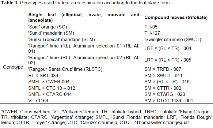
This study was conducted with 22 genotypes of Genetic Breeding Program of citrus (GBP Citrus) of the Embrapa Cassava and Fruits, being classified into two groups according to the leaf types: Simple and compound (Table 1). The leaves of each genotype were collected in five plants of each genotype cultivated in greenhouse during a year, in pots of 40 L.
Modeling and statistics of the results
From each genotype, 22 to 49 leaves were randomly collected sampling the maximum range of scope as possible. The leaf area of each leaf was determined using the methodology of Marshall (1968).
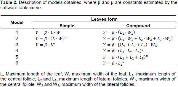
For the simple leaves, the maximum length of the leaf (L) and the maximum width of the leaf (W); for the compound leaves, the maximum lengths of the central folioles (L1) and lateral (L2 and L3) and the maximum widths of the central folioles (W1) and lateral (W2 and W3) were considered. Through the software Table curve, the biometric measurements were treated as independent variables and the leaf area as the dependent variable. The best models were selected based on the coefficient of determination (r2)(Table 2).
.
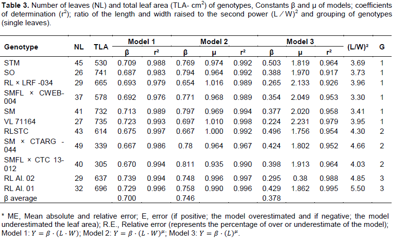
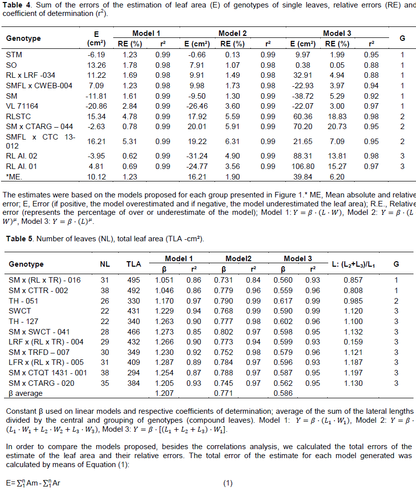
To increase the accuracy of the models for each type of leaf (simple and compound), they were separated into groups according to the form of the leaf blade. In the case of genotypes with single leaves, the criterion used was the relationship between the leaf length by its width (L/W) raised to the second power (L/W)², obtaining the groups: Group 1: 3 ≤ (L/W)2 ≥ 4; Group 2: 4.1 ≤ (L/W)2 ≥ 4.7, and Group 3: 4.8 ≤ (L/W)2 ≥ 6 (Table 3). For genotypes with compound leaves, was used the ratio between the sum of the length of lateral folioles and the length of the central folioles (L2+L3)/L1, with the formation of the following groups: Group 1: 0.8 ≤ (L2+L3)/L1 ≥ 0.89; Group 2: 0.9 ≤ (L2+L3)/L1 ≥ 1; Group 3: 1.1 ≤ (L2+L3)/L1 ≥ 1.3 (Tables 4 and 5).
In which E is the total error of estimate of leaf area (cm²); Am is the estimated leaf area (cm²); and Ar is the leaf area measurement (cm²).
The relative error was calculated by the ratio between the difference of the sum of the estimated leaf area (

) and the corresponding measured value ((

) by the sum of the real leaf area (

) (Equation 2):
In which RE is the relative error (%); (
) the sum of leaf area, of all the leaves in a genotype, estimated by the proposed model (cm²) and (
) the sum of leaf area, considering all the leaves in a genotype (cm²).
Adjusted models
The mathematical models presented the best adjustments were linear and potential, so they were selected for more detailed analysis. For genotypes with single leaves, three models were chosen: one linear and two potentials; for genotype with compound leaves, six were chosen: three linear and three potential (Table 2).
Models for genotypes with single leaves
All equations of the models individually generated for the genotypes possessing single leaves presented r2 above 0.9 (Table 3). The constant μ of Model 2 (simple leaf blade) tended to unity, showing that, regardless of the format of the leaf, leaf area is approximately 70% of the area of the rectangle (L.W), with no gains in accuracy with the use of the potential model. When only the length of the midribs as independent variable is used (model 3), the lowest value for constant μ was approximately 1.8, being characterized as potential (Table 3).
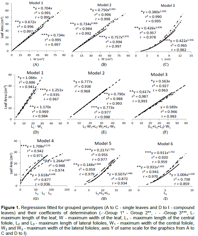
As shown in Figure 1, the adjusted models considering the three leaf groups (simple leaf), explained very well the variation of the data presenting excellent adjustment to mathematical models r2 ≥ 0.99. It was noticed a proximity to responses of the models when analyzing range in the abscissa axis corresponding to small leaves (L∙W ≤ 30 cm, L ≤ 5 cm) (Figure 1A to C). Consequently, the procedure of grouping, expressed by the ratio (L/W)2, promotes gains in estimates of LA, especially for larger leaves, range in which there is a greater dispersion of the models, regardless of the genotype tested. When considering the leaves grouping based on the relation (L/W)2, it was possible even the distinction of the access selected from a genotype, as the case of Rangpur lime (RL), in which the selections Aluminum 01 and 02 (group 3) belonged to distinct groups of Santa Cruz (RLSTC) (Group 2) (Table 3).

The estimate errors for each genotype, from the use of the adjusted models for each group (Figure 1), are presented in Table 4. In the case of the linear model (Y = β. (L.W )) they were lower in relation to the two powers (Models 2 and 3), with ER ranging from 0.62% to aluminum RL 02 to 5.31% for SMFL x CTC 13-012; and the average deviation the lowest among the three models tested (Table 4). The third model, in which it was used only the length (L) as the independent variable, proved to be comparatively less precise, especially for the genotypes belonging to groups 2 and 3. That result indicates the need of use of all the variables L and W in the estimates of single leaves for a greater precision regardless of the group. Considering that there were different responses depending on the genotype evaluated, with relative error (RE) minimum of 0.05% for SO and maximum of 20.73% for SM x CTARG - 044, proportionally different from the models which used L.W as input variable ï‚£ 6.31%. Among the models for simple leaf format, the most appropriate was the linear (Y = β. (L.W)). The advantages are by the high precision on the estimates and ease of practical application, confirming and justifying its widespread use in the estimate of leaf area in different plant species (Blanco and Folegatti, 2005; Coelho Filho et al., 2005, 2012, Cristofori et al., 2007; Malagi et al., 2010; Sousa et al., 2014; Souza and Amaral, 2015).
Models for compound leaves genotypes
The mathematical models tested fitted well for all genotypes, by the values of r2 ³0.84 (Tables 4 and 5). The choice of mathematics ratio (L2+L3)/L1, originally based on visual observations of variability, was attested by the high correlation with the constant β, model 1 (Table 5), Spearman’s correlation coefficient of 0.98 (figure not shown).
Considering only the linear models (Table 5), there was less variation in the amplitude of the values of the constant β in the third model proposed; therefore, the model was sensitive to changes in the shape of leaves. In a converse way, variations were greater for the first model. Such results probably reflect the number of variables used in each model.
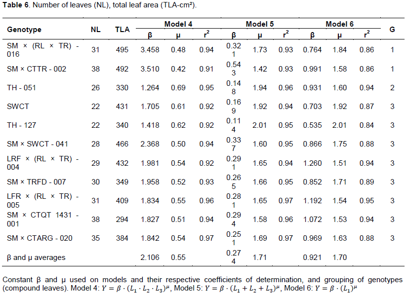
Analyzing the estimates of leaf area within each genotype, based on the adjusted models from each group (Figure 1), it was observed that the largest number of independent variables used in Model 2 reflected the higher values for the coefficient of determination, except in SM x (RL x TR) genotype - 016, in which it was noticed the best fit when using the third model (Table 5). Possibly the greatest number of independent variables of the model 2 increased its sensitivity, regardless of the leaf groups (1, 2 and 3), expressed by the proximity of the angular coefficients obtained (Figure 1E). That result suggested the feasibility of using an average value, regardless of grouping.
Considering that observation, a single regression with the data of 11 genotypes of compound leaves based on that model (
was performed. The value of β is equal to 0.776 and the model explained very well to the values observed by the coefficient of determination of 0.976 (figure not shown). In that case, in function of response independent of the genotype, the lack of concerning with groupings is a positive point. However, there is a need for a greater number of independent variables, which can restrict its use in practice, when the goal is to perform a large number of measures.
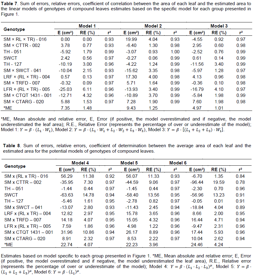
The proximity of the results with the use of linear models (Table 7) (average deviation of the relative error (RE) ranging from 1.01 to 1.48; and average deviation of error (E) ranging from 4.97 to 9.43), justifies the use of the Model 1
, due to its greater simplicity and practicality, confirming one more time the widespread use by different authors.
Analyzing the potential models, it was found that the constant μ for groups in the leaf model 4 (
were lower than one (Table 6), suggesting a reduction in the estimate rate of leaf area according to the increase of leaf length (Figure 1 G), what can cause major errors in the estimate of the area of leaves with high length. On fifth and sixth models, once the exponents are larger than the unit (Table 6), the angular coefficient of the tangent lines to the curve increases with the elevation of the value of the input variable, the opposite of what happened in the fourth model (Figure 1G to I).
Despite the high accuracy of the estimates obtained individually for the genotypes, in relation to the potential models 4, 5 and 6, according to the coefficients of determination (Table 8), when analyzing the statistical parameters ‘average error’ and ‘standard error’, there is a greater precision and accuracy when used with the linear models (Tables 7 and 8).
The greater precision of estimates is achieved when using specific models for each type (simple and compound leaves) and separating these types in homogeneous groups in relation to leaf dimensions and folioles. For simple and compound leaves, the respective linear models (Y = b. L. W; Y = b.L
1.W) showed the best statistical performance, besides being easy to use. The potential models Y= β L
µ and Y= β L1
µ, respectively for simple and compound leaves, require only one input biometric variable, which in a practical way, allow an increase in the number of repetitions, but provide errors of estimates higher than linear models. The model Y =
(L
1∙W
1+L
2∙W
2+L
3∙W
3) has been sensitive in the estimates of leaf area, independent of the grouping of compound leaves genotypes, for a
= 0.7755.
The authors have not declared any conflict of interests