Full Length Research Paper

ABSTRACT
Modeling the performance of an academic course based on a given set of affecting factors is the goal of this research. For different institutions, these factors differ in terms of availability and usefulness. This study was conducted for the nine engineering departments at King Abdulaziz University, Saudi Arabia with a total of 281 courses for the last 8 years. First, all measurable input factors were acquired from the database, and a comprehensive statistical study to course performance was performed. In modeling the input factors to the course performance, an adaptive linear model was first implemented at three levels: the college level, the department level, and the course level. Results show that the linear model fitted only 49% of the courses with an error standard deviation of 5.41 grade points, which is above the target of 2.5. On the other hand, the proposed neural network model showed much promising results: 83% of the courses were fitted with an error standard deviation of 0.96, having 95.26% of courses being modeled perfectly. In regard to the neural network structure and type, an exhaustive analysis was conducted by constructing and training 71,295 neural networks. It showed that the feed-forward and the cascade-forward types are the best with hidden layers between two to three.
Key words: Course performance, modeling, neural network, performance indicators, statistical testing.
INTRODUCTION
Many activities influence the success of an academic course; two are of a special nature: advising for registration and the continuous improvement of the course design. Both are controllable and can be tailored to every semester’s needs. First, however, it is important to study the aspects affecting the success of a course, students being the core of attention in this matter. In that, numerous factors contribute to the success of a course; yet in order to have an efficient and automated system, these factors must be:
1. collected objectively and reliably,
2. be available when needed,
3. and the process of acquiring them should be sustainable within the institution.
Once the factors have been decided for a given institution, their relationships with the course performance must then be modeled for evaluation. Knowledge of the individual factors is helpful in the general sense; however, a well-developed model would be more practical to improve the course performance. In this study, we highlight the most effective factors influencing the course performance for the Faculty of Engineering at King Abdulaziz University. Many approaches will be conducted, and their outcomes will be compared to find out the model that best relates the different effective factors of the course performance. Statistical analyses will also be carried out from different views for better understanding of the proposed model.
LITERATURE REVIEW
In searching the literature, one can find a number of studies relating different factors to academic performance. The work conducted by Winter and Dodou investigated the high school exam scores in relation to the academic performance at the freshman level in the engineering disciplines at the Dutch Technical University (Winter and Dodou, 2011). It shows that clustering high school courses into natural sciences and mathematics reflects the strongest predictor of the GPA. Similarly, in the Aviation College at the University of Tartu, a significant impact of the secondary school grades on academic performance is found, and that it should be set as a selection criterion (Luuk and Luuk, 2008).
Gallacher evaluated the practicability of using university admission tests as predictors of performance in under-graduate studies programs (Gallacher, 2007). The study concludes that admission tests are a useful predictor even if they are not comprehensive.
On the contrary, Thomas from the School of Physics, Georgia Institute of Technology showed that the performance of the diagnostic tests in the introductory physics course on the engineering students is a poor predictor of course performance, and that the students’ performance in the previous courses has a more significant correlation (Thomas, 1993). In fact, the study by Chamillard at the US Air Force Academy, Colorado Springs employed the students’ performance on previous courses to predict specific courses for curriculum improvement purposes (Chamillard, 2006). The prediction model used was a simple linear regression. Another study at the University of Technology in Jamaica shows that the performance of the first year computer science courses determines the academic performance and hence efforts should be invested in such subjects (Golding and Donaldson, 2006). Finally, a study at Coimbatore Institute of Technology in India listed a set of 7 attributes as key performance indicators to predict students’ pass/fail results. The list includes the secondary and high school percentages, subject difficulty, family income, medium, and staff approaches (Shana and Venkatachalam, 2011). Some of the attributes however were measured subjectively by surveys.
Other types of factors impacting the course performances are also found in literature. A study on 864 students was made at the Department of Economics, United Arab Emirates University. Results show that the most effective factors on performance are competency in English, students’ participation in class, and attendance (Harb and El-Shaarawi, 2009).
Another study on 304 students at North Carolina State University identifies some non-cognitive variables that predict first year students' academic performance. It reveals that developing a better understanding of how non-cognitive variables, such as emotional intelligence, relate to GPA and SAT scores is critical for future decisions of educational administrators (Jaeger et al., 2003).
While a lot of factors contribute to the performance of students, only the measureable and accessible ones would be feasible in maintaining a continuous monitoring system of the administration for better planning as well as to the instructors to objectively design their class activities. Input factors available in the information database will be considered in this study to model a course performance. For different institutions with possibly more accessible and reliable factors, we believe that the more incorporated input factors, the better the modeling results will be as will be shown in this paper. We first define the course performance as the average performance (grades) of its successful students excluding the failings, which might be considered at different research.
FACTORS AFFECTING COURSE PERFORMANCE
Course performance, or indeed the performance of the students registering a course, can be affected by many factors. As stated earlier, some of the factors can be measured and quantified while many others are difficult or impossible to measure or estimate (e.g. the un-predictable non-cognitive factors such as the emotional and the psychosocial). Thus achieving a comprehensive set of factors that influences the course performance is not our goal; though we believe that presenting as many measurable factors as possible for the administration and instructors would be more accurate in designing successful courses. The forthcoming factors were acquired from the database of the Faculty of Engineering at King Abdulaziz University, Jeddah, Saudi Arabia. For a given target course to be modeled at a given semester, the autonomously collected factors are:
Class Size: the total number of students registering the course
Students’ Loads: the statistics (mean and standard deviation) of the credit hours registered by the students in the class while taking the course under modeling. High mean value means the students in the class are over-loaded, and high standard deviation means the class is very diverse with students of low and high loads.
Students GPAs: the statistics of the students’ GPAs registering the course; again the higher the mean the better it is for the students, and high standard deviation means the class is more diverse in terms of GPA
Students’ Prerequisites Grades: the statistics of the prerequisite courses grades. If the course has more than one prerequisite course, the statistics is applied to the collective set (e.g. if 10 students are registering the course that has two prerequisites, then the set of the 20 prerequisite grades is considered for statistics)
Students’ Off-Plan Delays: the statistics of the number of semesters the students delayed taking the course according to their plans
Data were collected from the Fall-2005 until the Spring-2012 semester for the nine different programs at the college with a total of 281 different courses. The engineering programs are: aeronautical, civil, chemical, electrical, industrial, mechanical, thermal, mining, and nuclear engineering. The dataset has 4138 records; each record has the above mentioned input factors statistics (both mean and standard deviation) along with the actual course performance at the end of its semester. Table 1 shows the basic statistics of the input factors as well as the course performance (grades).
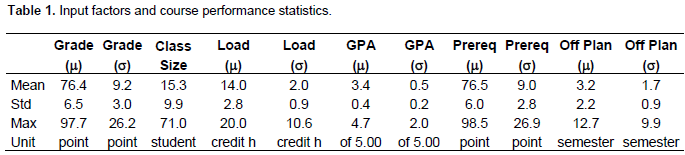
The mean value of the grades of the different courses of the college over the years is 76.4, which is a C+ grade letter. For the different courses, the grade mean value ranges from this mean with a standard deviation of 6.5, that is 69.9 to 82.9 is the 1-s confidence range. The second column of the table represents the variation of the students’ grades within a single course. If this number is zero, then all students got exactly the same grade in that specific course. Across all the college courses over the years of study, the course grade standard deviations averaged to 9.2 and reached 26.2 at a single occurrence, which is odd unless the class size is too large. The remaining columns of the table show the input factors statistics. For instant, the students are delaying taking their courses according to their plans by about 3.2 semesters. This number should be zero if all students took their courses as they were supposed to. At one course, this mean value reached 12.7 semesters, suggesting that a student in that course at some semester has delayed taking the course more than 7 years. In fact, the regulations prohibit students to stay more than 10 years to get their B.Sc. degrees.
The correlation coefficients between the course performance and the different input factors are also carried out for the entire dataset. Figure 1 shows how the input factors are statistically correlated to the course performance. Clearly, both the mean value of the course prerequisite grades and the average students GPAs have the most effect on the course performance. Class size has a correlation coefficient of +15% to the course performance. It was unexpected to be positively correlated; i.e., the larger the class size the better the students perform. However, the average class size is about 15 students, and one third of the college classes having less than 10 students. It might be seen that more students in a class would enrich the discussions and make the class active. A closer focus on this observation might be needed in a different study.
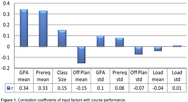
The next negatively impacting factor found was the students delays in taking their curriculum courses off their plans; the longer the students delay taking a course according to the plan the weaker the course performance is expected. The impact however is relatively low (10%). All other factors show almost insignificant correlation coefficients to the course performance, namely the variation of the students’ prerequisite grades, the variation of the students at their off plan delays, and the statistics of the students’ loads when taking the course of interest.
It is also useful to discuss some of the factors statistics for all records of the college. Table 2 shows the complete correlation coefficients of the input factors and the course performance.
The interesting relationships between the different input factors are discussed:
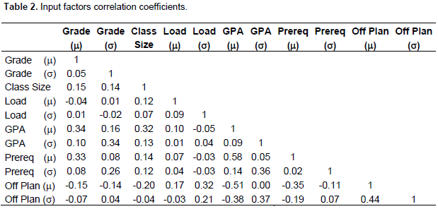
1. larger class sizes have higher GPA averages(-20%): it might show that good students with high GPAs and less off-plan delays tend to register in large classes
2. similarly, classes with high GPA students are having low off-plan delays (-51%) and less diverse too (-38%)
3. classes with students highly diverse in credit hours loads tend to have high off-plan delays (+32%) as well as very diverse students in off-plan delays (+21), yielding lower course performance
4. obviously, classes with students of high GPAs are having high average grades in the prerequisites (58%), and the more diverse class in terms of GPAs would be more diverse in the prerequisite grades (+36%)
In summary, the successful classes are the ones with high input GPA mean values, high prerequisite grades, low off-plan delays, and reasonable class sizes, which is no surprise.
PERFORMANCE MODELING
The simplest scheme to model a course performance as a function of input variables is to assume additive linear relationships with adjustable weights (Priestley, 1988). For n input variables, let a course performance, y, at a given semester of interest be modeled as:
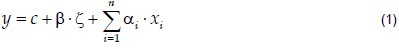
where, xi is the ith input factor affecting the course performance, ai is the dependence weight, z is an independent normalized random variable representing all non-modeled factors, b is the multiplicative factor of the normalized random variable, and c is the regression constant.
Before applying regression to estimate c, b, and ai’s, let us first calculate the correlation between the course performance and each input in order to identify the most important affecting factors; let mI be the mean value of the ith input factor xi, and si be its standard deviation based on the dataset prior to the semester of interest. The mean and variance of y will then be:
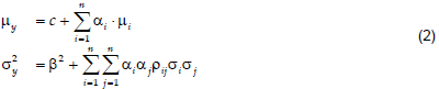
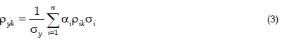
where rij is the correlation coefficient between inputs i and j. The correlation coefficient between y and any of the inputs xk is then:
In a matrix form, let:
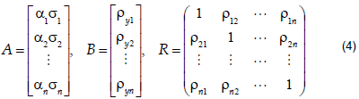
Then,

Given the correlation coefficients between the inputs, R, and between the output and any input, B, ai can be estimated for i from 1 to n as:

from which ai's are calculated; c and b, can be estimated from Equation (1), and hence:
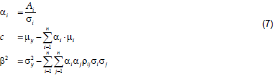
To sum up, for a given course, its performance can be modeled by calculating all of its affecting factors statistics (mi, si, and the correlation coefficients between them, rij’s) based on the dataset available. The statistics of the course performance from the dataset is then calculated, namely, my, sy, and ryi. Estimates of ai, c, and b are carried out using Equations (6) and (7). The modeled course performance can finally be calculated using Equation (1) where xi’s are the input factors evaluated for the registered students; b´z is the adjusting independent random quantity and will be eliminated from the model. Effectively however, b is an estimate of the standard deviation of the modeling error.
The parameters ai, c, and b can be estimated differently at three levels:
1. all college courses are evaluated in one model,
2. courses of each individual department have a model,
3. or each course has its own model separately
Neural network modeling
More effectively, one may utilize the dynamic learning property of the artificial neural networks in modeling the course performance. Since the discovery of the human brain function, artificial neural networks have been used to mimic the way our brains identify and predict events based on prior knowledge acquired (Krose and Smagt, 1996). A neural network consists of neurons which are small mathematical engines that sum some input signals from other neurons with certain weights and output a mapped activation function of the sum. The activation function of a neuron is a non-linear, monotonically increasing, continuous, differentiable and bounded function; the most commonly used are the sigmoid functions (Russell and Norvig, 1995):
.png)
where, y is the neuron output, xi are the inputs, wi are the weights of the inputs, b is the bias, and f(.) is the non-decreasing arbitrary activation function, a sigmoid function in this paper.
Neural networks are structured in layers, each having a number of neurons. The signal streams between the neurons of the different layers distinguish the network architecture, and the simplest neural network is the feed-forward where the outputs from the neurons in a given layer are fed only to the immediate next layer neurons as inputs. Figure 2 shows the neural network architectures used in this study.
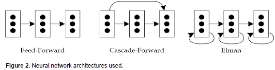
The activation function assigned to the different neurons is also a concern. Together with the size and structure of the network, one could obtain the best or the worst model for a specific problem. In general, the feed-forward networks are best used in classification applications such that used by (Sejnowski and Rosenberg, 1987) in converting English text to speech. Machine classification of sonar signals are also best modeled by feed-forward network, while the cascade-forward and the Elman networks are suitable for complex and large systems.
Regarding the network size in terms of the number of layers and neurons in each layer, an exhaustive search has been carried out in this study to compare the different networks and to decide the best model, starting by a single layer with neurons from 1 to 20, and up to three layers with combinations of neurons in each layer. These sets of networks were constructed and trained for the college courses first, and then for each of the 9 departments separately, and finally for the 281 courses. A total of 71,295 neural networks were simulated for this study.
MODELING RESULTS
Several basic calculations were first tried to compare with the two proposed models: the adaptive linear model and the neural network model. Considering the course performance statistics only, one may claim that the college or a department or even a course would retain its historical average performance without even considering any affecting input factor. For that claim, an error analysis was carried out to see the actual course performance in relation to its historical mean value. Results are as follows:
1. Considering the college’s mean value, which is 76.4, as the performance model for all courses in the college, the error statistics has a standard deviation of 6.5 grade points. Note that the error mean value is negligible and has no significant interpretation since some of the courses have positive errors while others have negative values. The standard deviation is our meaningful indication of the error size.
2. When considering each department of the college alone, i.e., each department having its mean value as the model to all of its courses, the performance errors have standard deviations ranging from 4.73 to 7.88 for the different departments.
3. Now considering each course alone regardless of its department, the error statistics in modeling the different courses is in the range from 1.05 to 13.52 points. Figure 3 shows these statistics.
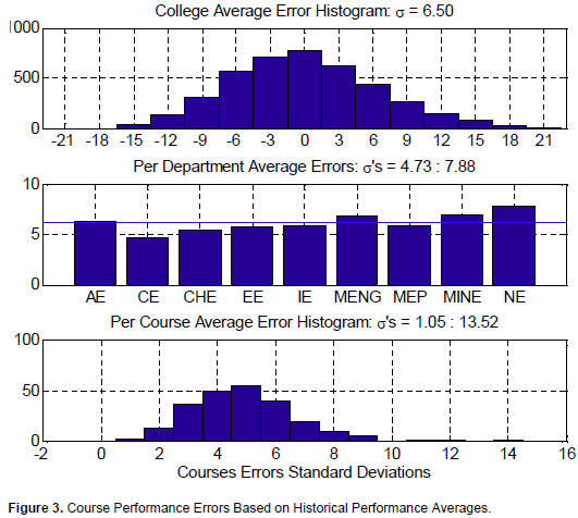
In summary, the best case scenario of the historical average based modeling has a standard deviation of 4.73 for one of the departments, and an average of 4.91 grade points among all courses when considering each course alone. These figures are now our reference for the model improvement.
Adaptive linear model results
When incorporating the abovementioned affecting factors in modeling the course performance, results show better modeling results. Figure 4 shows the modeling errors as follows:
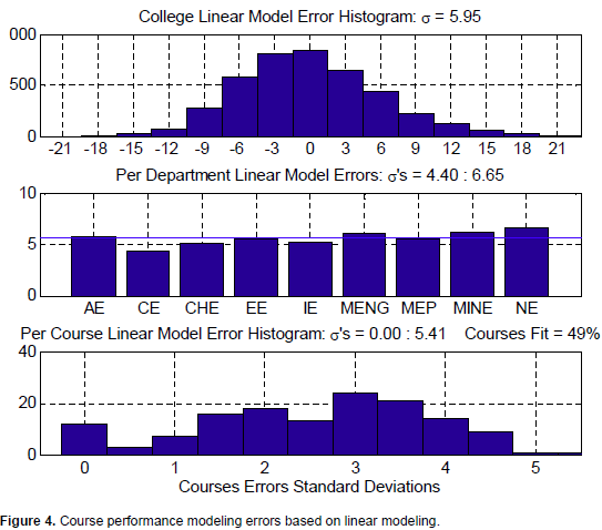
1. Fitting all the courses of the college into one linear model gives an error standard deviation of 5.95 points. This is an improvement of about 8% to simply taking the college average as a model of performance. The college linear model parameters are:
.png)
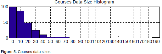
3. When it comes to fitting a linear model for each course alone, the overall error standard deviations are much better; they range from almost perfect modeling for some of the courses to 5.41 points in the worst case. However, only 49% of the courses fit the linear modeling while 51% fail to fit. Careful investigation reveals that the regression did not converge for these courses due to the few data points available. Since there are 9 input factors to fit the linear model, there should be at least 10 or more data points to fit. For the 281 courses in the database, 142 courses of them have fewer records than 10; thus could not be modeled. Figure 5 shows the histogram of the data sizes of the courses.
We might conclude that the linear model is better than the simple average model, whether considering the courses in the college, in their departments, or individually. Next we move to the hypothesis that information in the input affecting factors is not linearly correlated to the course performance. Modeling results of the neural network model follow.
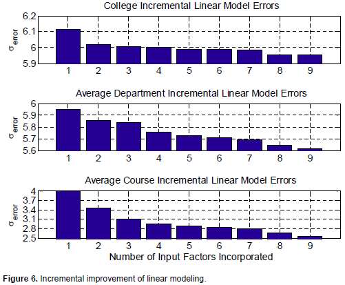
Incremental modeling results
In this section, we show the effectiveness of modeling when more input factors are considered. Figure 6 shows the linear modeling error standard deviation when adding more and more inputs. When considering only one input factor, namely the GPA mean average, the errors were the worst compared to the case where two input factors are considered, and so on.
Neural network model results
Similar approach is maintained in modeling course performance when treated at the college level, the department level, and individually. As stated earlier, a number of neural networks were configured and trained in each case, and the errors of the models were then reported. Results are shown in Figure 7:
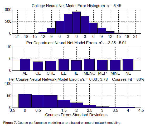
1. At the college level, the best neural network was the cascade-forward with two internal layers of sizes (9 and 3 neurons). The error standard deviation is 5.45, with about 8% improvement to the linear model, and 16% improvement to the historical average.
2. At the department level, each department has its own neural network, and the errors range from 3.85 to 5.04 points with better modeling than the adaptive linear.
3. When building a neural network for every course, results are of a much improved values.
On the average across the different courses, the modeling error is 0.96 points ranging from almost zero up to 3.78. With a target error of 2.5 grade points, 95.26% of the courses were modeled correctly, and the remaining 4.74% of the courses were modeled one letter grade off. Moreover, the neural network modeling was able to fit 83% of the courses unlike the linear modeling.
Analyzing the trained and simulated neural networks at the different levels, we find that 50% of the courses were best modeled by the CF neural networks type, 48% of the courses by the FF networks, and only 2% by the ELM type. Thus, the Elman neural network does not model the course performance of the affecting factors very well. Regarding the cascade- versus feed-forward types, we may conclude that courses behave similarly to either one.
Regarding the number of layers, we found that about 50% of the courses were best modeled by 2 hidden layers, while 38% of the courses were best modeled by 3 layers, while about 12% of the courses were modeled by only 1 hidden layer.
Finally, a comparative study was conducted on the total number of neurons of the networks to see how many neurons best fit the courses which are distributed among the hidden layers. Figure 8 shows a histogram of the best number of neurons for the different course models. The average is about 11 neurons ranging from as little as 2 to 20.
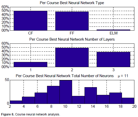
These observations suggest that in order to model the performance of a given course, a good start is to build either a feed-forward or a cascade-forward neural network with two hidden layers and a total of 11 neurons distributed randomly between the two layers. Variations of the model accuracy may then be observed at different configurations.
Analysis of variance
In order to objectively compare the accuracy of the linear and neural network models, we carried out some statistical tests to analyze the standard errors of the two models, namely the F-test (Christensen, 1996) and the Levene test (Levene, 1960). The difference between the two tests is that the F-test assumes both model errors are normally distributed. When the samples are not normally distributed, then the Levene test is a better nonparametric alternative. The F-test however gives more accurate results but when its condition is definitely satisfied.
Our hypothesis is that the error variance of the neural network model, is less than that of the linear model, . Thus, we set the null and alternative hypotheses as:
.png)
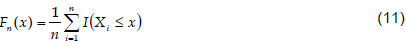
The first step is to test the normality of the modeling errors using the widely employed Kolmogorov-Smirnov goodness of fit test (Massey, 1951). To carry out this test, the empirical cumulative distribution function is calculated from the sample data points  as follows:
The Kolmogorov-Smirnov statistics (KS) is then:


For the F-test, the F-statistics value is computed as follows:
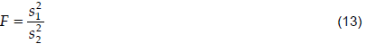
where  and
and  are the linear model and neural network samples variances, respectively. Traditionally, one sets a level of significance, say
  , and finds a Critical Value from the F-distribution tables based on that along with the degrees of freedom of the samples. A comparison is then made between the F-statistics and the Critical Value to give a decision whether to reject or accept the null hypothesis. However, modern computing tools are now more efficient to calculate the p-value directly from the samples. The p-value is simply the probability of the null hypothesis. The lower the p-value the more evidence to reject the null hypothesis; and it will be up to the reader to decide on the confidence level.
For the non-parametric Levene-test, the statistics value is calculated as follows:
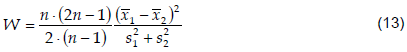
where and are the ith sample mean (or preferably the median) and variance, respectively. The p-value of the test is based on tabulated probabilities.
In this work, the course performance modeling was conducted at three levels: the college, the department, and the course level using both the linear and neural network modeling. In carrying out the analysis of variance statistics, the following steps were followed:
1. test the sample normality using Kolmogorov- Smirnov goodness of fit
2. compute the F-statistics if samples are normal at confidence level of 0.05
3. calculate the p-value of F-test
4. compute the p-value of Levene-test when either samples are not normal
5. report the decision on the null hypothesis
These steps are carried out for each of the three modeling levels. Figure 9 shows the Kolmogorov-Smirnov statistics calculated on the modeling errors to check for the normality of the model errors. It can be seen that both the linear and neural network the college models are not normally distributed. The p-value of the linear college model is 0.0000882, and 0.028 for the neural network model. These values are way below any acceptable confidence level to accept the normality hypothesis. Similarly, 56% of the neural network course model errors are not normally distributed considering a confidence level of 0.05. Thus, it is preferable to use a nonparametric Levene statistical test to compare the modeling errors distributions for both college and course levels, and to use F-test at the department level.
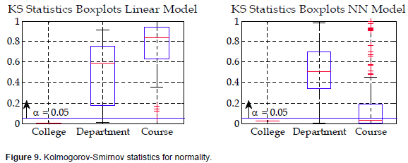
Figure 10 displays the p-values of both the F-tests and Levene-tests in boxplots at the different modeling levels:
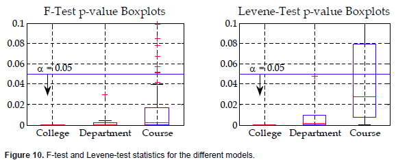
1. At the college level, the Levene-test is used yielding a p-value of 1.42x10⁻⁷ which indicates a strong rejection of the null hypothesis and accepting the alternative, that is, the two models having totally different distributions.
2. Similarly at the department level where 9 department models were compared, the p-values of the F-tests range from 6.3x10⁻⁸ to 0.0293, indicating that the linear and neural network models are also different.
3. At the course level, the F-tests and the Levene-tests are used according to the normality tests of the neural network course model errors.
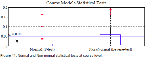
Figure 11 shows the p-values boxplots for the course models according to the normality tests, F-test when samples are normal, and Levene-test when samples are not normal. 77% of the normally distributed course models have significant different statistics of the linear and the neural network models, and 71% of the non-normal course models have different distributions for the linear and neural network. These percentages were found at a level confidence of 0.05. For the remaining percentages of course models, there is not enough evidence that the linear and neural network models differ from each other.
CONCLUSION
In this paper, we presented two modeling methods for an academic course performance based on a set of factors. The study considered those measurable quantitative factors that have noticeable correlation with the course performance and that of high availability. Results show nonlinear behaviors of the affecting factors when mapped to the course performance, thus modeling with a neural network would be more precise. Modeling improvements are attainable when more inputs factors are considered. The study shows that when adding more factors to the model, accuracy is increased. Thus for a given institution, the more factors considered, the better the modeling will be.
Modeling the course performance was performed at three different levels grouping courses in either individually, according to their departments or all together as one college model. While the adaptive linear model fitted only 49% of the courses with an error standard deviation of 5.41 grade points, the proposed neural network model was able to fit 83% of the courses with a small error standard deviation of less than one grade point.
Besides the average error observations, statistical tests were employed to objectively compare the accuracy of the linear and neural network models. Utilizing the F-test for normally distributed errors and Levene-test for the non-normal models, results show that the neural network models at the different levels have much lower standard errors than the linear models, confirming the nonlinear behavior of the course performance at all levels.
Although this study was mainly conducted for the courses of the Faculty of Engineering, King Abdulaziz University, other colleges and universities might benefit from similar modeling, especially the advantages of the neural network modeling for performance.
CONFLICT OF INTERESTS
The authors have not declared any conflict of interests.
ACKNOWLEDGEMENT
This work was funded by the Deanship of Scientific Research (DSR), King Abdulaziz University, Jeddah, under grant No (9-135-D1432). The authors acknowledge DSR’s technical and financial support.
REFERENCES
|
Chamillard AT (2006, June). Using Student Performance Predictions in a Computer Science Curriculum. Proceedings of the 11th Conference of the Innovation and Technology in Computer Science Education, Bologna, Italy. |
|
|
|
|
|
Christensen R (1996). Analysis of Variance, Design, and Regression: Applied Statistical Methods. Chapman & Hall, 1st Edition. |
|
|
|
|
|
Gallacher M (2007). Predicting Academic Performance. Social Science Research Network (pp. 1-16), Argentina. |
|
|
|
|
|
Golding P, Donaldson O (2006, October). Predicting Academic Performance. Proceedings of the 36th ASEE/IEEE Frontiers in Education Conference, San Diego, CA. |
|
|
|
|
|
Harb N, El-Shaarawi A (2009, February). Factors Affecting Students' Performance. J. Bus. Educ. 82(5):282-290. |
|
|
|
|
|
Jaeger A, Bresciani M, Ward C (2003, November). Predicting Persistence and Academic Performance of First Year Students: An Assessment of Emotional Intelligence and Non-Cognitive Variables. Association for the Study of Higher Education (ASHE) National Conference, Portland, OR. |
|
|
|
|
|
Krose B, der Smagt P (1996). An Introduction to Neural Networks. The University of Amsterdam Publications, 8th edition. |
|
|
|
|
|
Levene H (1960). Ingram Olkin, Harold Hotelling, et alia, ed. Contributions to Probability and Statistics: Essays in Honor of Harold Hotelling. Stanford University Press pp.278–292. |
|
|
|
|
|
Luuk A, Luuk K (2008). Predicting Students' Academic Performance in Aviation College from their Admission Test Results. Proceedings of the 28th Conference of the European Association for Aviation Psychology, Valencia, Spain. |
|
|
|
|
|
Massey F (1951). The Kolmogorov-Smirnov Test for Goodness of Fit. J. Am. Stat. Assoc. 46(253):68–78. |
|
|
|
|
|
Priestley M (1998). Non-Linear and Non-Stationary Time Series. Elsevier, 1st Edition |
|
|
|
|
|
Russell S, Norvig P (1995). Artificial Intelligence: A Modern Approach. Prentice-Hall, 1st Edition. |
|
|
|
|
|
Sejnowski T, Rosenberg C (1987). Parallel Networks that Learn to Pronounce English Text. Complex Systems 1:145-168. |
|
|
|
|
|
Shana J, Venkatachalam T (2011). Identifying Key Performance Indicators and Predicting the Result from Student Data. Int. J. Comput. Appl. 25(9):45-48. |
|
|
|
|
|
Thomas E (1993). Performance Prediction and Enhancement in an Introductory Physics Course for Engineers. J. Eng. Educ. 82(3):152-156. |
|
|
|
|
|
Winter J, Dodou D (2011). Predicting Academic Performance in Engineering Using High School Exam Scores. Int. J. Eng. Educ. 27(6):1343-1351. |
|
Copyright © 2024 Author(s) retain the copyright of this article.
This article is published under the terms of the Creative Commons Attribution License 4.0


