ABSTRACT
Inflation tends to be a relatively persistent process, which means that current and past values should be helpful in forecasting future inflation. Applying this intuition, we construct a basic stochastic model which exploits information embedded in past values of Ghana’s inflation data. Therefore the aim of this study is not to identify the drivers of Ghana’s inflation, but to identify and forecast with the best predicting model for Ghana’s inflation, based on the stochastic mechanisms that governs Ghana’s inflation series. We then use this identified model to forecast one-year-ahead (that is, 2018) inflation using past lags, specifically, monthly inflation, from January 2010 to September 2017. Per our forecast, the Bank of Ghana’s aim of hitting a single digit for the year 2018 will not be realized, even though the year closes with a lower inflation than what it began with.
Key words: Inflation, ARIMA model, forecasting, Ghana.
Inflation is defined as the increase in general price levels of goods and services within a period of time. Price stability, however, is a healthy monetary policy that promotes economic growth and prosperity. It is therefore not surprising that the primary objective of the Bank of Ghana (BOG) is to pursue sound monetary policies aimed at price stability and creating an enabling environment for sustainable economic growth. Price stability in this context, according to the BOG’s January 2017 Monetary Policy Summary report, is defined as a medium-term inflation target of 8% with a symmetric band of -2% or +2% at which the economy is expected to grow at a full potential without excessive inflation pressures. However, it is important to note that the extent to which inflation is anticipated can help in its control and hence the importance of inflation forecasts. Inflation forecasts are very important for policy makers, industries, businesses and institutions, just to mention a few, since pictures of the future serves as a guide for planning. According to Bailey (1956), the cost associated with unanticipated inflation includes the distributive effects from creditors to debtors, and also increasing uncertainty, which affects consumption, savings, borrowing and investment decisions.
The purpose of time series analysis is generally twofold: to understand or model the stochastic mechanism that has resulted in an observed series and to predict or forecast the future values of a series based on the history
of that series and, possibly, other related series or factors. The stochastic mechanisms that underlie a time series are helpful in explaining its evolutions; to be specific the autoregressive and moving average processes, and/or their composite forms. This paper sets out to empirically develop a linear dynamic stochastic model and apply it to forecast inflation for the year 2018. This model is based on the Box and Jenkins autoregressive integrated moving average (ARIMA) method.
The use of the ARIMA method in forecasting is essentially agnostic and unlike other methods that require the principles underlying an econometric model or structural relationships; it operates on the assumption that past values of a series plus its previous error terms contain information which can help in forecasting. According to Brent and Mehmet (2010) inflation tends to be a relatively persistent process, which means that current and past values should be helpful in forecasting future inflation.
Related works on Inflation using the ARIMA approach
Meyler et al. (1998) used the ARIMA model to forecast Irish inflation and justified that ARIMA models are surprisingly robust with respect to alternative multivariate models. Indeed, Stockton and Glassman (1987), upon finding similar results for the United States’ inflation forecasts, commented that “it seems somewhat distressing that a simple ARIMA model of inflation should turn in such a respectable forecast performance relative to the theoretically based specifications”. Okafor and Shaibu (2013) modelled Nigeria’s inflation employing quarterly data which span from the year 1981 to 2010. They realized ARIMA (2, 2, 3) as the most appropriate and used it to provide forecasts. Okyere and Mensah (2014) made forecasts of Ghana’s inflation for the year 2014 using the Box Jenkins approach. They employed monthly data from January 2009 to December 2013. They realized ARIMA (1, 2, 1) as the most appropriate for modelling inflation. Suleman and Sarpong (2012) used monthly inflation data covering the periods between January 1990 and January 2012, to model and forecast Ghana’s inflation. They realized ARIMA(3,1,3)(2,1,1) (Sinaj, 2014) as the best model to define Ghana’s inflation evolutions.
This study was carried out in Ghana in the year 2017 using monthly inflation data for the periods between January 2010 and September 2017. The data were obtained from the Bank of Ghana’s website. The data were modelled using the ARIMA stochastic model.
Autoregressive integrated moving average (ARIMA) model
A time series {Yt} is said to follow the ARIMA model if the dth difference Wt = ∇dYt is a stationary ARMA process. If {Wt} follows the autoregressive moving average model, that is, the ARMA (p, q) model, we say that {Yt} is an ARIMA (p, d, q) process, where is the order of the autoregressive (AR) component, is the number of differences needed to arrive at a stationary ARMA (p, q) process, and is the order of the moving average (MA) component. The general form of the ARIMA model is represented by the backward shift operator,
∅(B)(1 – B)dYt = θ (B)et, (1)
where
∅(B) is the AR characteristic polynomial evaluated at B, and is expressed as:
∅(B) = (1 - ∅1B - ∅2B2 - --- - ∅pBp) (2)
θ(B) is the MA characteristic polynomial evaluated at B and is also expressed as:
θ(B) = (1 - θ1B - θ2B2 - --- - θqBq) (3)
∅ is the parameter estimate of the AR component
θ is the parameter estimate of the MA component
∇ is the difference
B is the back shift operator
et is a purely random process with mean zero where var(et) = σ2e and
(1 – B)dYt = ∇dYt (4)
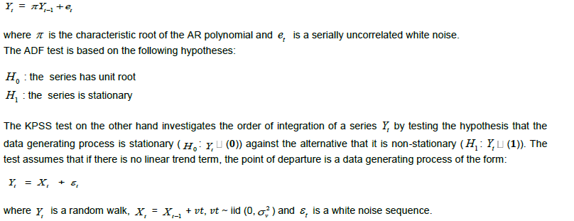
Unit root test
It is very important to ensure that a time series is stationary before making inferences about it. The basic idea of stationarity is that the probability laws that govern the behavior of a process do not change over time. The Augmented Dickey Fuller (ADF) test, proposed by Dickey and Fuller (1979) and the Kwiatkowski-Phillips-Schmidt-Shin (KPSS) test proposed by Kwiatkowski et al (1992) were employed to check for stationarity in this study. The ADF test is based on the assumption that a time series data follows a random walk:
Thus the KPSS tests to see if stationarity can be rejected, which is the reverse of the ADF test.
Model building
Finding the appropriate model for a time series involves a multistep model-building strategy as espoused by Box and Jenkins. There are three main steps in the process, each of which may be used several times:
(i) Model specification (or identification)
(ii) Model fitting, and
(iii) Model diagnostics
Model specification
This is the stage where models that may be appropriate for an observed series are selected. The model at this stage is only tentative and subject to revision later on in the analysis. Bad choices of parameters for any ARIMA (p,d,q) model leads to bad forecasts. But it is also worthy of notice that a good model does not necessarily produce a good forecast. We employed three selection criteria in this study to provide guidance for selection of possible models: The Akaike Information Criterion (AIC), the modified Akaike Information Criterion (AICc), and the Bayesian Information Criterion (BIC). The (AIC) was proposed by Akaike (1974). For any of these criteria, the model which has a lower score receives recommendation for consideration.
Model fitting
Model fitting consists of finding the best possible estimates of
unknown parameters within the specified ARIMA models. The maximum likelihood procedure is used to estimate the model parameters. The maximum likelihood procedure is a flexible way of estimating models. Most econometric data are observational and that can complicate analysis since observationally identical individuals can respond differently to a similar situation, and vice versa. Given the specified model, the maximum likelihood procedure among others, addresses such problems by producing the best possible measurements, using all information provided in the data.
Diagnostic checking
The fit of the ARIMA (p,d,q) model with the estimated coefficients is checked at this stage. This involves the scrutinization of the estimated residuals to ensure that they behave approximately like the realizations of a white noise process. For a good model, the residuals must be white noise. Statistical tools such as the Ljung-Box test, proposed by Ljung and Box (1978) and also the ACF plots of the residuals were used to check model adequacy in this study.
Stationarity
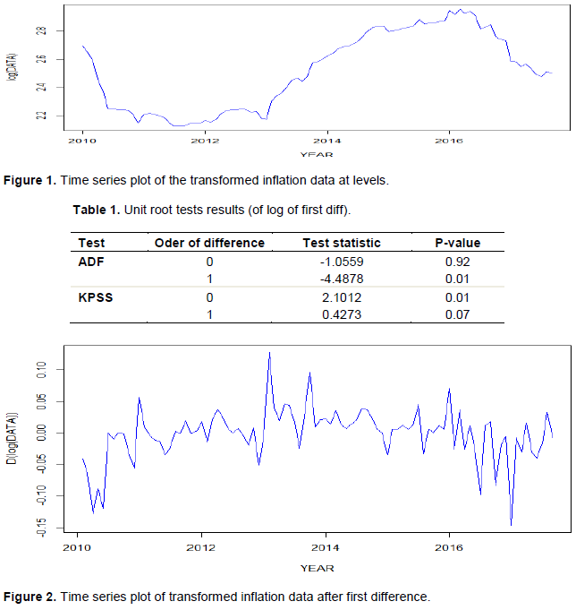
Figure 1 shows time series plot of the data from January 2010 to September 2017. Clearly the data are not stationary at levels. The ADF and KPSS tests results in Table 1 confirm the non-stationarity of the series at levels. The data however attained stationarity at first difference as seen in Table 1 and Figure 2. In Table 1 it can be seen that the p-value associated with the ADF test at levels (that is, at order of difference 0) is more than 0.05. It can also be seen that the KPSS test at levels has an associated p-value of less than 0.05, and in all cases, this is an indication of non-stationarity. When the associated p-value of an ADF test is less than 0.05 as seen for the first order of difference in Table 1, it is an indication of stationarity, but for the KPSS test, a p-value of more than 0.05 is rather an indication of stationarity. Before taking the first difference, we did a logarithm transformation of the data so as to eliminate any possible distortions of heteroscedasticity.
Model identification
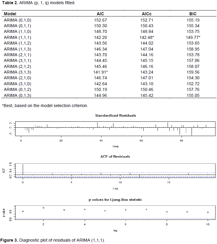
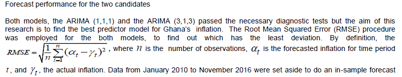
Literature suggests several ways of determining the number of lags to include in a model. The drawback is that, for the same data, a different method can yield a different order. Considering this disadvantage, we used trial and error approach to model fourteen proposed models as shown in Table 2. A rough idea of parsimonious upper bounds can however be provided by the ACF and PACF plots of the stationary series. As mentioned earlier we used the AIC, AICc, and the BIC selection criteria to guide our selection of possible candidates among these proposed models. ARIMA (1,1,1) was recommended by both AICc and BIC, but the AIC criterion suggested ARIMA (3,1,3). Therefore ARIMA (1,1,1) and ARIMA (3,1,3) were tentatively selected at this stage to undergo model estimation and diagnostic tests.
Model diagnostics
We decided to carry out the diagnostics before we estimate the parameters since in our case more than one model received recommendations and the idea was to carry out the diagnostics first, so that we do not waste any time estimating the parameters of a model which fails the diagnostic test. And so diagnostics were carried out to confirm the proposed ARIMA (1,1,1) and ARIMA (3,1,3) models.
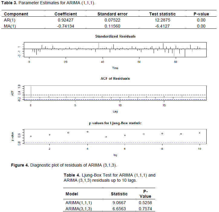
It can be seen from the ACF plots of the residuals in Figure 3 that the ARIMA (1,1,1) residuals are white noise although there is a significant spike at lag 0. Furthermore, the graphical and numerical p-values of the Ljung-Box Test respectively displayed in Figure 3 and Table 3 confirms the model adequacy of the ARIMA(1,1,1). The ACF plots of the residuals in Figure 4 and the Ljung-Box results in Table 4 below shows that there were no serial correlations for ARIMA (3,1,3) as well, which proves that the ARIMA (3,1,3) is also adequate for analyses.
Model estimation
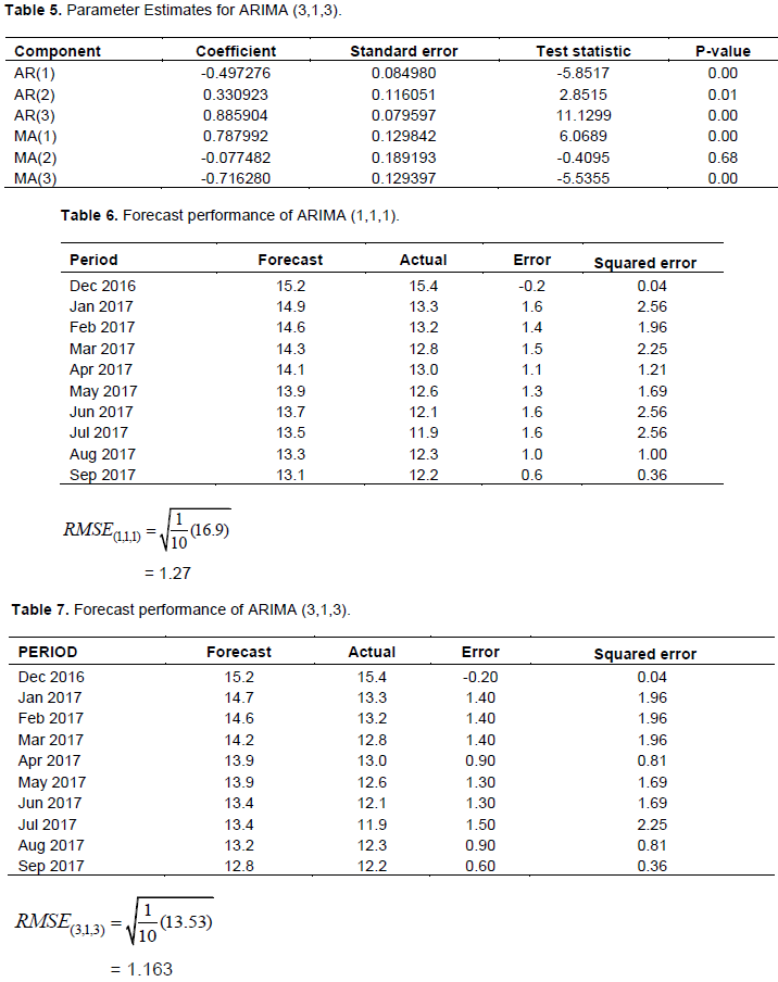
The maximum likelihood procedure was used to estimate the model parameters of ARIMA (1,1,1) and ARIMA (3,1,3) and the results is as shown in Tables 5 and 6. As seen from Table 3, all parameters are significant for the ARIMA (1,1,1), but for the ARIMA (3,1,3) model, the MA (2) parameter is not significant as shown in Table 4.
for the period between December 2016 to September, 2017. This helped in estimating the forecast performance of the two models as shown in Table 7 using the RMSE procedure.
Both models passed all the necessary diagnostic tests, and even though the ARIMA (1,1,1) had two recom-mendations, it was outperformed in the forecasts by the ARIMA (3,1,3) which had only one recommendation. Since the aim of this study is to find out the best predictor model, we settle for the ARIMA (3,1,3). This establishes that the evolution of Ghana’s inflation is a weighted sum of its past three values plus its past three error terms. Lubowa et al (2014) modelled and forecast Uganda’s inflation and also realized ARIMA (3,1,3) as the most appropriate model. Valentina (2014) also realized ARIMA (3,1,3) as the best model in her work “models to forecast in Albania”. In her work, she used the ARIMA model to forecast inflation, whilst she used the multivariate vector autoregressive (VAR) model to identify the drivers of inflation in Albania. She employed only the AIC in the determination of the best ARIMA model. The equation of an ARIMA (3,1,3) model is of the form:
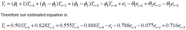
We suggest that in order to do any meaningful analyses for inflation for any particular month, the Bank of Ghana needs to consider inflation values within the immediate past three months and also the error terms of those past three months. It can also be seen from the estimated equation for ARIMA (3,1,3) above that the past two values of inflation has more explanations than that of any other month. As per our forecast (Appendix Table 1), even though inflation is expected to reduce, the Bank of Ghana’s aim of hitting a single digit inflation cannot be realized in the year 2018. In view of this, the bank of Ghana should review their economic policy.
The authors have not declared any conflict of interests.
REFERENCES
|
Akaike H (1974). A New Look at Statistical Model Identification. IEEE Transactions on Automatic Control 19:716-723.
Crossref
|
|
|
|
Brent M, Mehmet P (2010). Simple ways to forecast inflation: What works best? Trade Publication 17:1-9.
|
|
|
|
|
Bailey JM (1956). The welfare cost of inflationary finance. Journal of political economy 64:93-110.
Crossref
|
|
|
|
|
Dickey D, Fuller W (1979). Distribution of the Estimates for Autoregressive Time Series with a Unit Root. Journal of the American Statistical Association 74:427-31.
|
|
|
|
|
Kwiatkowski D, Phillips PCB, Schmidt P, Shin Y (1992). Testing the Null Hypothesis of Stationarity against the Alternative of a Unit-root; How sure are we that Economic Time Series have a unit-root? Journal of Econometrics 54:159-178.
Crossref
|
|
|
|
|
Ljung G, Box G (1978). On a Measure of Lack of Fit in Time Series Models, Biometrika 66:67-72.
Crossref
|
|
|
|
|
Lubowa W, Wokadala J, Nyanzi MT (2014). Modelling and forecasting inflation in Uganda (2005-2014). International Journal of Sustainable Economy 9(2):121-141.
Crossref
|
|
|
|
|
Meyler A, Kenny G, Quin T (1998). Forecasting Irish inflation in using ARIMA models. Technical Paper 3(98):85-102
|
|
|
|
|
Okafor C, Shaibu I (2013). Application of Arima Models to Nigerian Inflation Dynamics. Research Journal of Finance and Accounting 4(3):2222-1697 (Paper), 2222-2847 (Online).
|
|
|
|
|
Okyere F, Mensah C (2014). Empirical Modelling and Model Selection for Forecasting Monthly Inflation of Ghana. Mathematical Theory and Modeling 4(3):99-106.
|
|
|
|
|
Sulema N, Sarpong S (2012). Empirical approach to modelling and forecasting inflation in Ghana. Current Research Journal of Economics Theory 4(3):83-87.
|
|
|
|
|
Sinaj V (2014). Models to forecast inflation in Albania. International Journal of Scientific Research 5(1):2229-5518.
|
|