The purpose of this study is to investigate the stability of money demand function in emerging countries using the annual data over the period 1987 to 2018. The panel data was analyzed applying both static and dynamic panel models. With the static panel analysis, the random effect method is found to be an appropriate model to determine the factors that affect money demand in emerging countries. The findings of random effect method reveal real income affect money demand positively while exchange rate and real interest rate influence money demand negatively. The results of dynamic panel approach show that real income has positive impact on broad money demand while exchange rate, real interest rate and inflation negatively influence broad money demand in the long-run. The dynamic panel approach confirms that inflation has a significant impact on money demand in addition to the variables found to significantly influence money demand with the random effect method of static panel approach. This implies that dynamic panel model better estimates the determinants of money demand function as compared to static panel model. The stability analysis of each country confirms stable money demand function. The error correction model reveals any deviation from the equilibrium is corrected each year in the selected emerging countries. Therefore, the monetary policy makers can incorporate the outcome of this study as additional input for the implementation of effective monetary policy in the selected countries of emerging economies.
Money provides a trade-off between the liquidity benefit of holding money and the interest advantage of holding working and fixed assets. The demand for money is a desire and ability to decide in which way people can accumulate their wealth. Economists explain the money demand as the choice of keeping the financial assets in the form of money; either as cash or bank demand deposits. Money is demanded not for its own sake, but for all the functions that it can perform. Money demand theory seeks the reasons for why both individuals and institutions would like to keep a part of their income on hand and how much of it, and the reflections of this behavior on the economy. The stability of money demand ensures predictability of the variables, and therefore reduces the possibility of an inflation bias. That means a stable money demand articulates that the changes in the elements of money demand equation can be predicted. The stability of money demand function reveals the variables that determine the quantity of demanded money remain consistent over time period. Stable money demand exists if the demand for money has a long-run cointegrating association with its determinants without any systematic changes in the regression coefï¬cients.
The determinants and stability of money demand are two crucial concepts in the theory of money demand. While the classic quantity theory of Fisher underlines income as the only determinant of the money demand function, Keynes and Friedman consider the variables such as interest rates, bond and equity returns, and the return on physical goods in addition to output (Diu and Donald, 2010). Kjosevski (2013) explains a stable money demand function as the quantity of money is predictably associated to a set of key variables connecting money to the economic real sector. Understanding the stability of money demand and its determinants is the key functions in formulating appropriate monetary policy for countries considering a monetary targeting framework. In other words, discussing the money demand function is the main target for monetary policy makers since the combination of money supply and money demand decides the interest rate, and hence influences the aims of monetary policy (Oscalik, 2014).
In case that the money demand function is stable, the authorities can change the money supply in order to eliminate economic stagnation or fight against inflation. In the case of achieving a stable money demand function which can be explained by variables such as income, interest rate, inflation expectation; it is possible that the increase in the money supply may affect those variables in the expected way, the money demand could reach the new level of money supply and the money market could find the balance again (Rao and Kumar, 2008). The determinants and the stability of money demand play a crucial role in constructing efficient monetary policies for the market. Effective monetary policies can be made with the help of a stable and predictable money demand. With the expectation of stable money demand function, the policy makers considered monetary targeting as a successful strategy to attain price stability. However, the experiences of developed countries that pursued monetary targeting policy reveal the money demand function is not as stable as expected. Particularly, diversifying the financial instruments, increasing financial liberalization, regulatory changes in the banking sector and technological innovations related to the electronical payments required to reconsider the stability of money demand after the end of 1980s (Tumturk, 2017). In some countries the fundamental changes occurred in financial markets have affected the existence of stable relationship between the goal variables and targeted aggregate. Hence, the monetary authorities have reviewed the money demand function as “unstable” in the corresponding countries.
Emerging countries are not independent from the countries in which all these fundamental changes occurred in the financial markets. As Li (2014) states before the 1978 economic reform in China nearly all financial institutions combined into the People’s Bank of China (PBC), which served as the administration headquarter as well as the business center of China’s financial and banking system. PBC had exclusively controlled the money supply and also served as government treasury. However, in 1978 Chinese Communist Party reformed the structure focusing on a shift from “class struggle” to “economic development.” In the second half of 1980s, the PBC was transformed into the Central Bank of China to carry out monetary policy independently. The exclusive functions of the banking system as both administrative and commercial were finally separated. In the 1990s, the reform focused on creating an efficient banking system to formulate and implement monetary policy and issue loans being free from the control of the political orders.
Financial reforms have been implemented globally from the early 1980s although it is not able to state that all countries implemented these reforms with the same speed and at the same time (Rao and Kumar, 2008). India also implemented financial reforms in 1980s (Rao and Kumar, 2008; Singh and Pandey, 2009) where income elasticity has declined from 1.29 to 1.02 and the coefficient of interest rate, which was insignificant during 1970-1985 has become significant during 1985 – 2005 (Rao and Kumar, 2008). In 1990s Turkish financial markets also practiced deregulation and financial liberalization (Tumturk, 2017).
South Africa adopted the money market-oriented monetary policy measures in 1980s (Nell, 1999). In 2000 the country adopted an official inflation-targeting framework eliminating the monetary policy framework of setting predetermined targets for broad money (M3). However, this official monetary framework does not necessarily understate the significance of money in the formulation of an effective policy strategy, as long as stable money demand function exists and also the appropriate monetary aggregate (M3) comprises information about the future price changes (Nell, 2003). Stability of money demand function is a fundamental concept in macroeconomics as the appropriate design of the monetary policy is contingent upon the presence of stable money demand function (Tumturk, 2017). An important question to be raised is “Have the money demands been stable in the emerging countries?”
Several empirical researches have been carried out on money demand function in emerging countries based on the country specific data over the past few decades using various approaches. According to Hurn and Muscatelli (1992), some previous studies on money demand function using different approaches show that the function was stable over time. However, these studies fail to appropriately describe the existence of long-run relationship between money demand and its determinants. As Diu and Donald (2010) explain the estimates of money demand functions with various specifications fail to reveal a stable money demand function in several countries due to the structural changes like deregulation and financial innovations. The purpose of this study is therefore to address the question of which form of money demand function is appropriate for empirical work in emerging countries, and to determine whether or not the long-run cointegration exists between money demand and its determinants. Estimation of the appropriate functional form is crucial since the stability of money demand is contingent upon the established functional form.
This study contributes to the literature in determining the appropriate money demand function for emerging countries using both static and dynamic panel models. In addition, with time series analysis this study examines the stability of money demand function for group-specific countries using cumulative sum (CUSUM) and cumulative sum of square (CUSUMSQ) tests for the specified money demand function. The aim of CUSUM and CUSUMSQ tests is to find out whether the fundamental changes in financial market structure have compromised the stability of money demand function and changed the consistency of estimated coefficients. Hence, this study contributes to the literature on the determination of the stability of money demand function in emerging countries: Brazil, China, India, Indonesia, South Africa and Turkey using time series and panel approaches. The remaining part of the article is organized as follows. Section two presents some reviews of theoretical and empirical literature on the stability of money demand function. With the aim of determining stable money demand, this section reviews the empirical literature on most widely used models (cointegration and error correction modeling) and the application of CUSUM and CUSUMSQ tests. Section three elaborates the methodology followed in the investigation of the stability of money demand function. This section briefly describes the error correction model and cumulative sum test. Section four analyses the results of static panel approach with random effect method and dynamic panels with pooled mean group on the determinants of money demand function. This section also investigates the cointegration and stability of money demand function across countries: Brazil, China, India, Indonesia, South Africa and Turkey using the error correction models and stability diagnostic tests: CUSUM and CUSUMSQ tests. Finally, conclusions are provided based on the results of this specific study.
Demand for money has become temporarily unstable in developed countries after the financial reforms (Rao and Kumar, 2008). This is attributed to the effects of deregulation of the financial markets which has increased competition in the financial markets, created additional money substitutes, increased use of credit cards and electronic money transfers, increased liquidity of the fixed deposits and induced higher international capital mobility (Rao and Kumar, 2008; Diu and Donald, 2010). On monetary policy aspect, it forced many industrial countries to shift from the monetary aggregate targeting to inflation targeting policy framework. However, recently this view has changed as many empirical findings with various data definitions and econometric methodology have confirmed stable money demand function. According to Bahmani-Oskooee and Rehman (2005), money demand function in many Asian countries of developing economies is stable, in which case Central Banks target on money supply. It is necessary to investigate whether money demand function is stable or not since targeting on the interest-rate is inappropriate in the existence of stable demand for money (Rao and Kumar, 2008). This implies that stability of money demand function has implication on the choice of monetary policy instruments.
The stability of money demand function
Estimating a stable money demand function is essential for the Central Banks with respect to their targets on sustainable growth and price stability. Using panel data, Rao and Kumar (2008) find long-run relationship between money demand and the determinants: GDP and interest-rate for the selected Asian countries. In the study of comparing backward and forward looking approaches to modeling money demand in Turkey, the analysis of M2 broad money demand for the period 1980:Q1-1991:Q2 with quarterly data confirms that inflationary expectation is the most dominant factor affecting money demand. This implies that the expectations of economic agents adjust the inflation rate extensively, which allows them to put away inflation tax by reducing their monetary holdings (Saatcioglu and Korap, 2005).
Tumturk (2017) states that provided the average economic growth rate and nominal interest rate, monetary growth rate can be adjusted conformable with the price stability. Such adjustment is possible on condition of strong and stable relationship between inflation and targeted monetary aggregate. However, in the absence of strong and stable association between inflation and the targeted monetary aggregates, targeting on monetary aggregate is not applicable as experienced by a number of industrial countries. In other words, the weak and unstable relationship fails to give the anticipated outcome on inflation, and no longer will the targeted monetary aggregate provide a reasonable indication about the viewpoint of monetary policy (Mishkin, 1998). In Vietnam the empirical studies were carried out on the determinants of demand for money within the context of dollarization and underdeveloped financial markets, where the US dollar provides a substitute for the local currency. The findings reveal the cointegrating relationships among the variables: money-demand, output, real price stock and foreign interest rate. In addition, real money demand is sensitive to inflation. In this country the demand for real money was found to be stable over the period 1999 – 2009, and this is a vital foundation for the implementation of the appropriate monetary policy (Diu and Donald, 2010).
In Turkey, the bound test is applied in combination with CUSUMSQ test to analyze the stability of broad money demand with quarterly data over the period 1985:Q4-2006:Q4. The findings indicate the existence of stable association between money demand (M2) and the determinants: real-income, interest-rate and exchange-rate (Tumturk, 2017). Investigating the money demand function over the period 1989:Q1-2010:Q4, Gencer and Arisoy (2013) reveal the existence of long-run relationship between real-money demand and the determinants: real-income, exchange-rate, inflation and interest-rate in the Turkish economy. The findings show positive effect of real-income and exchange-rate on real-money demand while interest-rate and inflation negatively influence the real-money demand.
In the investigation of a stable long-run equilibrium association between money demand (M2) and the determinants: real-income, interest-rate, exchange-rate and inflation, Niyimbanira (2013) finds stable money demand function, and concludes effective monetary policy in South Africa based on results of the Error Correction model (ECM). In the determination of the stability of M3 money demand in South Africa, Nell (2003) finds stable money demand function over the period 1968 – 1997. In the analysis of the stability of the money demand function with a VAR-based approach in South Africa, Kapingura (2014) reveals the existence of cointegration between money-demand function and its determinants over the period 1994-2012 with quarterly data.
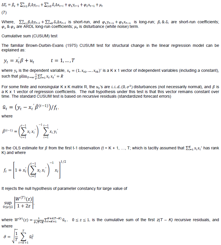
Cumulative sum and cumulative sum of square tests for stability
Many studies interpret the cointegration of monetary aggregate with income and interest-rate as a sign of stable demand for money. However, cointegration does not necessarily imply reliability of estimated coefficients. According to Bahman-Oskooee and Wang (2007), there are cases where the variables included in money demand function become cointegrated while the estimated money demand function remains unstable. This implies that cointegration is not sufficient for stability, and therefore it is necessary to test the stability of the specified money demand function using cumulative sum (CUSUM) of recursive residuals and cumulative sum of squares of recursive residuals (CUSUMSQ) tests to effectively determine whether or not the long-run and short-run estimated elasticities are stable over the specified time period.
Nduka et al. (2013) apply CUSUM and CUSUMSQ tests to investigate the existence of stable demand for money in Nigeria. The cointegration and stability findings confirm the existence of stable and long-run association between money demand and its determinants. The empirical findings reveal income and foreign-interest-rate influence the money demand positively while domestic-real-interest-rate, inflation-rate, and exchange-rate affect the money demand negatively. Okonkwo et al. (2014) explain that money demand function in Nigeria is stable as confirmed by CUSUM and CUSUMSQ tests. The coefficient of error correction term is negative and significant confirming the deviation from the equilibrium is adjusted towards the equilibrium.
Money demand functions of the emerging countries were investigated using both time series and panel data. The advantage of using time series over cross section data can be explained as the ability of investigating the dynamic relationships of the variables where the time series provide sufficient information about the earlier time period (Abonazel, 2016). The advantage of panel datasets over the individual time series includes the capability of controlling the unobserved heterogeneity in individuals/countries and increasing the degree of freedom for stable parameter estimation (Mitic et al., 2017). In other words, panel data do not only increase the total number of observations and their variation but also reduce the noise coming from the individual time series. Hence, heteroscedasticity is not an issue in panel data analysis.
In panel data analysis both the static panel and dynamic panel variants were considered for the investigation of the stability of money demand function. Static panel considers only exogenous variables as explanatory variables, while the dynamic panel variations include the lagged dependent variables as additional explanatory variables.
Static panel data model
Hausman (1978) test for selection of the appropriate estimator
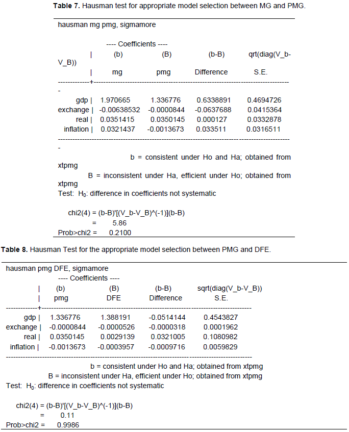
For the analysis of money demand function using dynamic panel data model, the Hausman test was performed to identify the efficient estimator among the estimators: Pooled Mean Group (PMG), Mean Group (MG), and Dynamic Fixed Effect (DFE). The hypothesis of the Hausman test can be described as follows.
(i) To determine the appropriate estimator between Mean Group (MG) and Pooled Mean Group (PMG), the null hypothesis of homogeneity can be described as:
H0: PMG is the most efficient estimate
H1: MG is the most efficient estimate
The p-value (0.2100) is greater than 5%, and we fail to reject the null hypothesis. Hence, the model supports the PMG estimator.
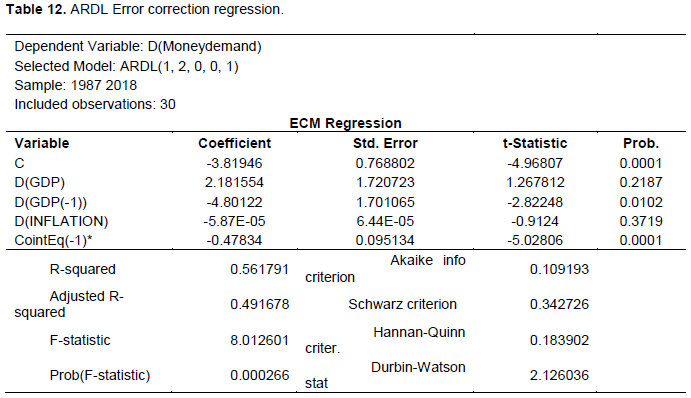
(ii) After finding that PMG was the appropriate estimator in comparison to MG, Hausman test was again performed to identify a suitable estimator comparing PMG with DFE. The hypothesis of Hausman test can be stated as:
H0: PMG is the most efficient estimate
H1: DFE is the most efficient estimate
The p-value (0.9986) is greater than 5%. So, we fail to reject the null hypothesis. Since the Hausman test confirmed the PMG as the most efficient estimate compared to MG and DFE, the dynamic panel analysis of money demand function was based on the PMG estimator, which was proposed by Pesaran et al. (1999). PMG is an intermediate estimator between MG and DFE. It allows the intercepts, short-run coefficients, and error variances to differ freely across groups, i.e. all these are heterogeneous. The PMG estimators are consistent and efficient under the assumption of long-run slope homogeneity. That means long-run coefficients are homogenous. In other words, PMG constrains the long-run coefficients to be identical, but allows the short-run coefficients and error variances to differ across groups. PMG generates consistent estimates of the mean of short-run coefficients by taking the sample average of individual unit coefficients.
Autoregressive Distributed Lag (ARDL) model for time series analysis
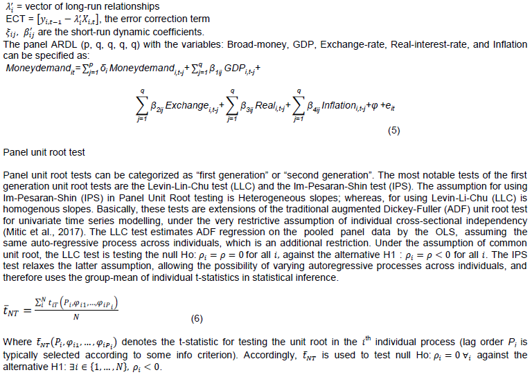
To investigate the stability of money demand function in each country of the panel members, the ARDL model was employed based on the results of the unit root test where some variables were integrated of order one, I(1), while some other variables were stationary at level, that is, I(0). The ARDL model can be specified as:
Source of data and description of variables
The study of money demand function was based on the annual data of period 1987 to 2018. The data were obtained from World Bank except the interest-rate data for Turkey which was obtained from Federal Reserve Economic Data (FRED). The classical quantity theory of Fisher describes income as the only determinant of money demand while other economists including Keynes, Tobin and Friedman explain the money demand function considering additional determinants: interest-rates, the return on physical goods, and bond and equity returns (Diu and Donald, 2010). Sichei and Kamau (2012) state that money demand functions can be effectively determined by including more determinants into the specification rather than the traditional specification. Hence, many variables were considered for efficient specification of money demand function for the emerging countries. The data for Money-demand and GDP were in natural logarithmic form; whereas, real interest rate, exchange rate and inflation were in percentages.
Money demand
it stands for broad money demand. Broad money was chosen to be dependent variable. It was measured in constant US dollar. The term broad money is used to describe M2, M3 or M4, depending on the local practice. The exact definitions of the three measures depend on the country. In China broad money M2 refers to the entire stock of liquid assets in an economy, such as cash and current account deposits, as well as “near money” indicators that are less liquid, such as savings deposits. According to Hurn and Muscatelli (1992), M3 is the highest money balance in South African monetary policy targets. M3 includes M2 plus longer-term time deposits and money market funds with more than 24-hour maturity. M4 includes M3 plus other deposits. Broad money is superior to narrow money in macroeconomic analysis. M0 and M1, also called narrow money, normally include coins and notes in circulation and other money equivalents that are easily convertible into cash.
Gross domestic product (GDP)
It stands for real income which was measured as GDP at constant prices. As Tumturk (2017) explains theoretically the sign of the income elasticity of money demand is expected to be positive. Hurn and Muscatelli (1992) also found positive relationship between GPD and real M3. Therefore, the sign for real GDP was expected to be positive.
Exchange
It stands for exchange rate. According to Kjosevski and Petkovski (2017), exchange rate plays a vital role in explaining money demand. Namely, during periods of high inflation, countries might experience a partial replacement of domestic with foreign currencies, either as a store of value or as a medium of exchange. According to Bitrus (2011), the return on the holdings of foreign assets is influenced by the expectation of exchange rate movements. That means depreciation of the domestic currency relative to foreign currencies would lead to a rise in the return on foreign assets to domestic holders and vice versa. Some findings state that when the exchange rate increases, the demand for money decreases. In such a case the exchange rate is inversely related to the demand for money while others including Gencer and Arisoy (2013) and Diu and Donald (2010) attach positive sign for exchange rate in relation to money demand. Hence, the sign for this variable was indeterminate a priori.
Real
It stands for real interest rate. Keynesians highlight the negative sign of interest rates with the significant effect on money demand (Diu and Donald, 2010). Zuo and Park (2011) also find negative effect of real interest rate on money demand in China. The sign for this variable was therefore expected to be negative.
Inflation
A priori expectation for the coefficient of inflation was negative. Diu and Donald (2010) find inflation to be negative in determining the demand for money in Vietnam. Niyimbanira (2013) states that many empirical findings in South Africa reveal negative effect of inflation on real money demand.
This study investigates the determinants and stability of money demand in emerging countries with the annual data of period 1987 to 2018. The random effect model was employed to determine the factors that affect money demand in emerging countries with the static panel analysis. The ARDL models were applied to investigate money demand function with dynamic panel approach and time series analysis. The stability test was performed for each country using cumulative sum of recursive residuals (CUSUM) and cumulative sum of squares of recursive residuals (CUSUMSQ) tests.
Static panel analysis
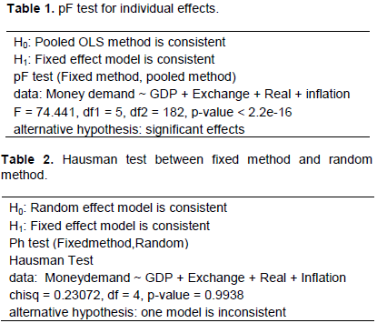
For static panel analysis, random effect model was found to be an appropriate model compared to pooled model and Fixed effect model based on the pFtest and Hausman test. The null hypothesis of “pooled OLS method is consistent” was rejected following the p-value (0.0000), which is less than 5% (Table 1). This test supports the Fixed effect model rejecting the pooled model.
Once the pFtest confirmed the fixed effect method as an appropriate model, this method was again compared with the random effect method using the Hausman test to investigate whether fixed effect method would be preferred to random effect method. However, the Hausman test supported the random effect as a consistent method since the p-value (0.9938) was greater than 5% (Table 2). So, the null hypothesis of “random effect model is consistent” was not rejected by the Hausman test. With static panel approach, money demand of emerging countries was, therefore, analyzed using the random effect method. The findings reflect that money demand in emerging countries is positively influenced by real income while exchange rate and real interest rate affect money demand negatively (Equation 8).

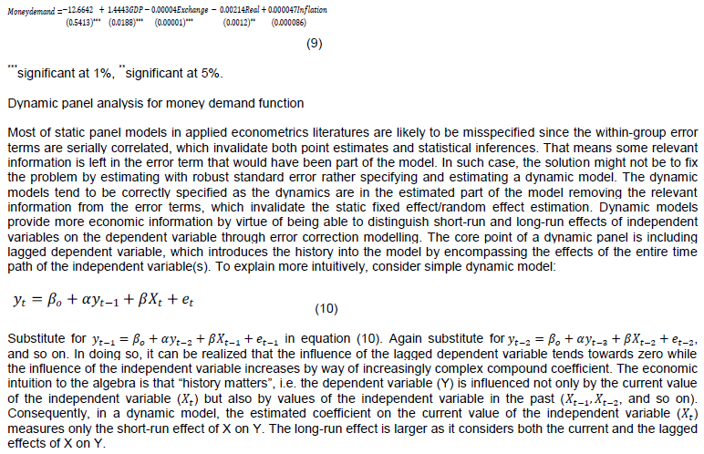
Real-income and exchange-rate are significant at 1% significance level while real-interest-rate is significant at 5% significance level. The findings reflect that a 1% increase in real income results in 1.44% increase in money demand in emerging countries. The exchange-rate and real-interest-rate negatively affect the money demand but the magnitudes are small, which are 0.00004% and 0.00213% change on money demand for 1% changes in exchange-rate and real-interest-rate, respectively.
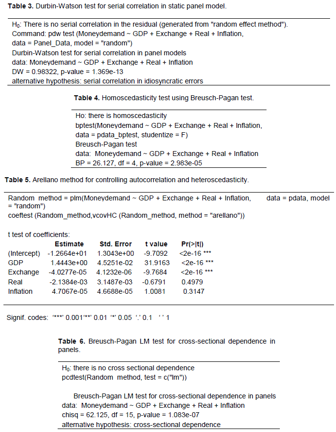
Most of the time in static panel data model the serial correlation problem is experienced due to misspecification by including only exogenous variables as the explanatory variables in money demand function. The serial correlation problem was checked by Durbin-Watson (DW) test. The null hypothesis of DW test is no serial correlation in the residual generated from random effect method. Since the p-value (0.0000) is less than 5%, we reject the null hypothesis of no serial correlation in favor of the alternative hypothesis that the model specification is serially correlated (Table 3). The random effect method was also checked for the heteroscedasticity of the data set using Breusch-Pagan test. The null hypothesis of the Breusch-Pagan test is that there is homoscedasticity in the data set. Since the p-value (0.0000) of the test is less than 5%, the null hypothesis of homoscedasticity is rejected in favor of the alternative hypothesis of heteroscedasticity in the data set (Table 4).
Durbin-Watson test for serial correlation and Breusch-Pagan test for heteroscedasticity confirmed that the static panel data model was suffering from both serial correlation and heteroscedasticity problem. To control the autocorrelation and heteroscedasticity of panel data, Arellano method was applied to make the standard error robust (Table 5). The results of Arellano method reflect that GDP and exchange rate are significant at 1%. However, real interest rate is found to be insignificant after controlling the heteroscedasticity and autocorrelation of the panel data. Similar to serial correlation in time series, cross-sectional dependence reduces the efficiency of least squares estimators, and invalidates conventional t-tests and F-tests which use standard variance-covariance (Baltagi et al., 2012; Kao and Liu, 2014). To detect the cross sectional dependence, the standard Breusch-Pagan LM test is applied when the number of cross-section (N) is less than the number of time periods (T) (Baltagi et al., 2012). The null hypothesis of the Breusch-Pagan LM test for cross-sectional dependence in panels can be stated as there is no cross-sectional dependence in the panels. The p-value (0.0000) of the test indicates the presence of the cross-sectional dependence (Table 6).
Cross sectional dependence can be corrected using Feasible Generalized Least Square (FGLS) and Panel Corrected Standard Error (PCSE). FGLS is preferred to PCSE when the time period (T) is greater than the cross section (N) in correcting the problem of cross sectional dependence. Whereas, PCSE is used when the cross section (N) is greater than the number of time series (T). Since the number of time series (T) of this study was greater than the number of cross section (Appendix B), the cross sectional dependence was corrected using the FGLS. FGLS is sometimes called Estimated Generalized Least Square (EGLS). Equation 9, in which cross section dependence is controlled by using FGLS, reflects that GDP influences money demand positively while exchange rate and real interest rate possess negative impact on money demand in emerging countries.

Hausman test was again applied to decide the best model between PMG and DFE with the null hypothesis that PMG was the most efficient estimate. The p-value (0.9986), which was greater than 5%, supported the PMG model as the efficient estimate (Table 8). That means the Hausman test confirmed Pooled Mean Group (PMG) as an appropriate model to investigate money demand function in emerging countries based on the balanced annual panel data over the period 1987 to 2018. PMG takes the cointegration form of a simple ARDL model and adopted for panel setting by allowing the intercepts, short-run coefficients and cointegrated terms differ across cross-sections. That means PMG allows intercepts, short-run coefficients and error variances to differ across groups while long-run coefficients are the same for all panel members. Pesaran et al. (1999) explain the long-run coefficients being the same across groups as common technologies influence all groups in a similar way. For example, Solow growth model often assumes the same technology across countries and hence long-run production function parameters would be the same though the speed of convergence to the steady state might vary based on different population growth rates across countries.
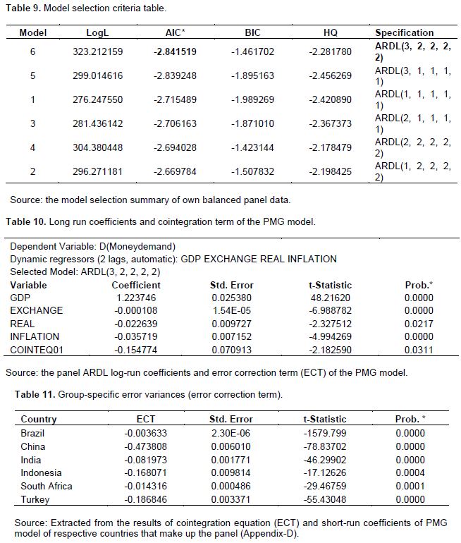
The panel model selection summary revealed ARDL (3, 2, 2, 2, 2) was the best lag structure, which had the lowest value (-2.841519) of Akaike Information Criteria (AIC) (Table 9). The dynamic panel analysis was therefore based on ARDL (3, 2, 2, 2, 2). The panel ARDL (3, 2, 2, 2, 2) model reflects that the long-run coefficients of each of the regressors are significant (Table 10; Appendix C). The elasticity of GDP is 1.22 and significant at 1% significance level. Exchange rate and inflation are also significant at 1% significance level and their elasticities are -0.0001 and -0.0357, respectively. The elasticity of real-interest-rate is -0.0226 and significant at 5% significance level. In the long-run, real income has positive impact on broad money demand while exchange-rate, real-interest-rate and inflation negatively influence broad money demand in the long-run. The negative effect of inflation rate on broad money supports the theoretical expectation that as the inflation rate rises, the demand for money falls. This indicates that people prefer to substitute physical assets for money balances. Rao and Kumar (2008) find that income elasticity of demand is about unity, and demand for money responds negatively to variations in the short term interest rate. Cointegration equation coefficient (-0.1548) is significant at 5% of significance level (Table 10), which confirms the existence of long-run relationship among the variables in the panel. This implies that any deviation from the long-run equilibrium is corrected at the speed of 15.5%.
The long-run coefficients are the same (homogenous) for all countries under the panel while their respective short-run coefficients differ across countries in the panel. This is because the assumption of Pooled Mean Group (PMG) is that only the long-run coefficients are the same for all the groups that make up the panel while each country (group member) has its respective error variances and short-run coefficients. The error correction term for Brazil reveals the deviation from the long-run equilibrium is corrected at the speed of 0.36%. Similarly, the deviations from the long-run equilibrium are corrected at the speed of 47.4, 8.2, 16.8, 1.4, and 18.7% for China, India, Indonesia, South Africa, and Turkey, respectively (Table 11).
Time series analysis for stability of money demand function
The diagnostic tests for stability, serial correlation and residual distribution were performed considering the group-specific regressions, which assume all coefficients and variances differ. With the specification of ARDL (3, 2, 2, 2, 2), the residuals were not normally distributed in time series of Brazil, and serial correlation was detected with such specification of time series in India, Indonesia and South Africa (Appendix D).
Pesaran et al. (1999) explain that the group-specific estimates are biased because of sample-specific omitted variables or measurement errors that are correlated with the regressors. Rao and Kumar (2008) state that it is difficult to introduce country-specific special factors in the panel data methods. In this study, such bias was corrected by experimenting with different specification of the model as ARDL (1, 2, 0, 0, 1) for Brazil; ARDL (3, 0, 0, 0, 0) for India; ARDL (2, 2, 2, 2, 2) for Indonesia; and ARDL (1, 2, 0, 0, 0) for South Africa. Whereas, in China and Turkey the group-specific estimates with ARDL (3, 2, 2, 2, 2) model reflected that the residuals were normally distributed, and no evidences of serial correlations were found in the model.
This confirmed the reasonable estimates with the model ARDL (3, 2, 2, 2, 2) for China and Turkey.
Stability of money demand function in Brazil
Money demand function in Brazil reveals the existence of cointegration between money demand and the determinants: GDP, Exchange rate, Real interest rate and Inflation (Table 12).
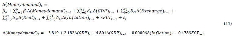
The negative sign of the coefficient of cointegration equation (-0.478341) reflects that if there is departure in one direction, the correction would have to pull back to the other direction so as to ensure that equilibrium is retained. The findings can be interpreted as the previous years’ deviation from the long-run equilibrium is corrected at the speed of 47.8%.
Diagnostic test for serial correlation and residual distribution
The result of Breusch-Godfrey serial correlation LM test reflects the higher p-value of chi-square (0.1722), which reveals no evidence for serial correlation of the model. Normality test for residual distribution also reflects that the p-value of Jarque-Bera is 0.4139, which is greater than 5%, and we cannot reject the null hypothesis that states the residuals are normally distributed. That means the normality test confirms that the residuals are normally distributed, and hence the model is correctly specified to determine money demand function in Brazil.
Test for dynamically stability of the model
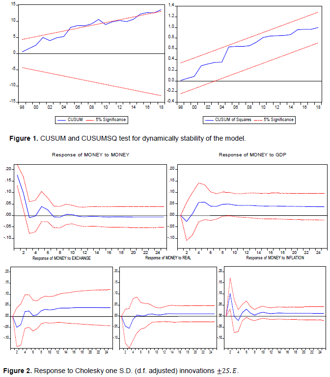
The CUSUM test shows that the blue line is deviated from the 5% critical boundary between 2005 and 2010 (Figure 1). This structural break reflects that Brazil experienced challenges related to the slowdown in advanced economies following the global financial crisis and the falling of Chinese demand for Brazilian commodities (Costa, 2016). However, the CUSUM of squares test reflects that the blue trend line lies within the red lines, which confirms that the model is dynamically stable. This finding reveals Brazil has quickly recovered from the global financial crisis. Although the recursive error in the CUSUM test slightly crosses the 5% upper critical limit between 2005 and 2010, the CUSUMSQ test shows greater stability. This confirms that the demand for money in Brazil by and large is stable.
Impulse response functions and variance decomposition
Impulse response function is defined as the change in the current and expected values of a variable (or a vector of variables) conditional on the realization of a shock at a point in time. It shows the effects of shocks on the adjustment path of the variables. Impulse response function determines how long and to what degree a shock of a given equation has on all of the variables in the system. Impulse response functions are able to explain the sign of the relationships as well as how long these effects require to take place. A useful insight is that an impulse response function is essentially just a plot of the coefficients of the moving average representation of a time series. The analogy of the impulse response is like dropping a stone in a pond, in which at first ripples will be bigger but as time passes, the ripples get smaller and smaller until equilibrium is restored. That means when a dependent variable experiences a shock, it will return to equilibrium over a period of time. Figure 2 illustrates how money-demand reacts to a shock to the variables: money-demand, GDP, Exchange-rate, Real-interest-rate, and Inflation. The response of a shock to money-demand is a positive in money-demand but it turns to be negative after year three though it immediately turns back to positive after year four, and then decreases until it finally dies out over time. This is the response of money-demand to a shock of itself. The response of money-demand to a shock of GDP is negative but after year three it becomes positive where the effect remains positive and remains constant over time period. Similarly, response of money-demand to shocks of exchange-rate and real-interest-rate is that first it becomes negative and after year four the effect becomes positive and constant.
Variance decomposition (forecast error variance decomposition) measures the contribution of each type of shock to the forecast error variance. It gives the proportion of the movement in the dependent variable that is due to its own shock versus shocks to the other variables. In other words, variance decomposition informs what fraction of the forecast error variance of a variable is due to different shocks, potentially at different horizons. It gives information about the relative importance of its shock to the variables in the VAR. In money demand function of Brazil, the percent of broad-money variance due to broad-money decreases sharply in the first two years and after the second year, the effect decreases gently.
The proportion of the movements of the money-demand, that is, its own shock versus shocks to GDP and exchange-rate increases while it becomes constant to shocks to real-interest-rate and inflation after year two (Figure 3). Hence, variance decomposition and impulse response analysis help to check the impact of one variable on the other.
Stability of money demand function in China
The bound test in money demand function of China reflects the existence of cointegration between money demand and its determinants. The error correction term (-0.07068) is negative and significant at 1% significance level, which can be interpreted as any deviation from the equilibrium is corrected at the speed of 7.1% each year (Table 13).
Serial correlation and normality test
The serial correlation diagnostics was carried out with the null hypothesis of no serial correlation in the residuals. The p-value of chi-square (0.1437) is greater than 5%, which confirms no evidence for serial correlation in the model specification. The normality test confirms the residuals are normally distributed since the null hypothesis of “residuals are normally distributed” is not rejected due to higher p-value of Jarque-Bera (0.598935).
Stability diagnostics
The stability diagnostics show that the blue lines are within the red lines boundaries for both CUSUM and CUSUMSQ tests, which confirm stable money demand in China (Figure 4). In the analysis of stability of money demand in China over the period 1983-2002 with the quarterly data, Bahman-Oskooee and Wang (2007) find that only M1 is stable with CUSUM and CUSUMSQ tests though both M1 and M2 are cointegrated with their determinants. The instability of M2 can be explained as in the second half of 1980s the People’s Bank of China was transformed into the Central Bank of China to carry out monetary policy independently (Li, 2014), which might cause the structural break over the period 1983 - 1987.
After the financial reforms, CUSUM and CUSUMSQ tests confirm stable money demand in China over the period 1987 – 2018.
Stability of money demand function in India
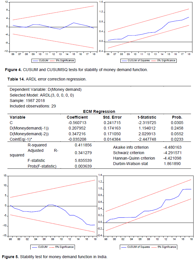
The negative sign of error correction term (ECT) reflects the convergence in the long-run if there is any deviation from the equilibrium. The coefficient of ECT (-0.035208) implies that the deviation from the equilibrium is corrected at the speed of 3.5% each year (Table 14). Money demand has cointegration with the determinants: GDP, exchange rate, real interest rate and inflation.
Diagnostics for serial correlation and normality test
Breusch-Godfrey serial correlation test was performed to detect serial correlation in the model with the hypothesis:
H0: there is no serial correlation
H1: the residuals are serially correlated
Since the p-vale (0.7828) is greater than 5%, the null hypothesis is not rejected. This implies that there is no evidence for serial correlation in the model. The normality test for residual distribution determines whether the residuals are normally distributed or not. The null hypothesis of the normality test is that the residuals are normally distributed. Since the p-value of Jarque-Bera is greater than 5%, which is 0.335522, we failed to reject the null hypothesis. This implies that the residuals are normally distributed.
Stability test for money demand function in India
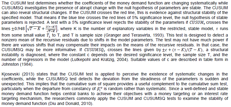
The CUSUM test determines whether the coefficients of the money demand function are changing systematically, while CUSUMSQ investigates the presence of abrupt change with the null hypothesis of parameters are stable. The CUSUM can also reveal structural changes. If the CUSUM crosses the red line, this is evidence against structural stability of the specified model. That means if the blue line crosses the red lines of 5% significance level, the null hypothesis of stable parameters is rejected. Since the blue line is within the red line boundaries (Figure 5), we fail to reject the null hypothesis. This implies that the money demand in India is stable. This finding is consistent with that of Rao and Kumar (2008) who state that there is no evidence that the long-run relationship between money demand and its determinants is significantly affected over the period 1985 to 2005. Bahmani-Oskooee and Rehman (2005) also state that demand for money is fairly stable in many Asian countries including India. In the investigation of stable money demand function after reforms, Nitin and Asghar (2016) find stable money demand function in India with monthly data over the period 1991 – 2014 using the cointegration and error correction model.
Stability of money demand function in Indonesia
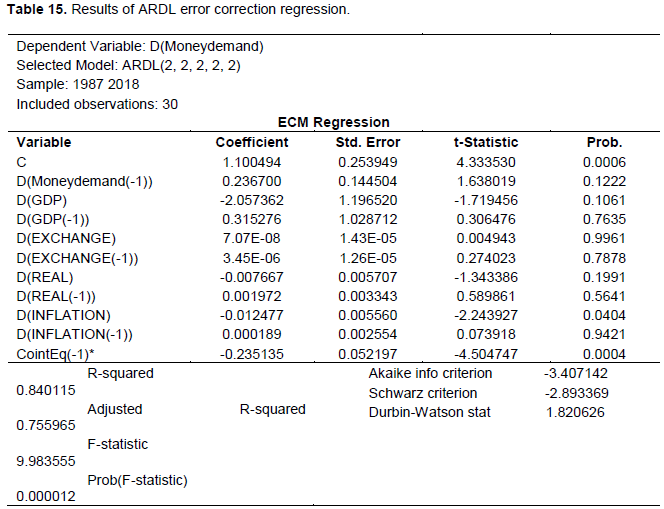
Money demand function in Indonesia reveals the existence of cointegration between money demand and the determinants: GDP, Exchange rate, Real interest rate and Inflation. In the analysis of the Indonesian influential factors of money demand, Prawoto (2010) also confirms the existence of long-run relationship between money demand and its determinants. The Error Correction Model (Table 15) can be specified as:
The error correction term (-0.2351) implies that the deviation from the equilibrium is corrected at the speed of 23.5% each year.
Diagnostics for serial correlation and residual distribution
The result of Breusch-Godfrey LM test reflects the higher p-value of chi-square (0.5951). This supports the null hypothesis of no serial correlation in the model. This implies that there is no evidence of serial correlation in the model. The normality test determines whether the residuals are normally distributed or not with the null hypothesis of the residuals are normally distributed. The higher p-value of Jarque-Bera (0.9720), which is greater than 5%, supports the null hypothesis. This confirms that the residuals are normally distributed.
Stability test for money demand function in Indonesia
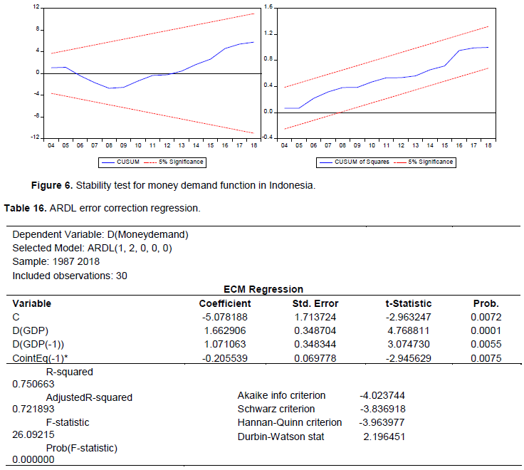
The CUSUM and CUSUMSQ testes were applied to detect the coefficients of the money demand function were structurally stable with the null hypothesis of parameters are stable. Figure 6, in which the blue line lies within the red line boundaries, implies that the money demand function in Indonesia is stable. Lestano et al. (2011) investigate money demand stability for Indonesia using both broad and narrow money demand equation over the period, 1980Q1-2004Q4. The findings reflect the existence of long-run relationships between broad and narrow money demand and their determinants. However, the CUSUM and CUSUMSQ tests reveal only narrow money demand is stable in Indonesia. They justify why broad money was not stable over the period 1980 – 2004 as that period was influenced by many financial liberalization including the financial crisis of 1997-1998. In addition to this justification, in their analysis the inflation factor was not considered in the specification of broad money demand function. This might also reflect unreliable result in the stability tests due to misspecification of the determinants. In the analysis of stability of narrow money demand in Indonesia, Hossain (2011) states that the narrow money demand is stable irrespective of ongoing financial reforms in Indonesia since the late 1980s. The findings also reflect the existence of long-run relationships between narrow money demand and the determinants: real income and the deposit interest rate.
Stability of money demand function in South Africa
The bound test in money demand function of South Africa reveals the existence of long-run relationship between money demand and its determinants. The error correction term (-0.2055) is negative and significant at 1% significance level, which implies that any deviation from the equilibrium is corrected at the speed of 20.55% each year (Table 16).
Diagnostics for serial correlation and residual distribution
The Breusch-Godfrey LM test was performed with null hypothesis of no serial correlation. The higher p-value of chi-square (0.5033), which is greater than 5%, supports the null hypothesis. This implies that there is no evidence of serial correlation in the model. The normality test was performed to investigate whether the residuals were normally distributed or not with the null hypothesis of “the residuals are normally distributed”. The higher p-value of Jarque-Bera (0.9588), which is greater than 5%, supports the null hypothesis. This implies that the residuals are normally distributed.
Stability test for money demand function
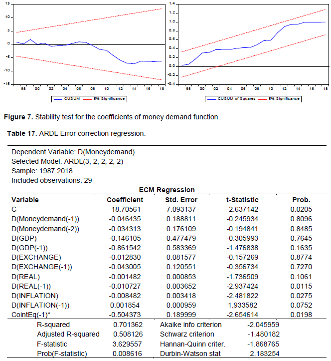
The CUSUM and CUSUMSQ tests were applied to investigate the stability of the coefficients of money demand function with the null hypothesis of stable parameters. Figure 7, in which the blue lines lie within the red line boundaries, implies that money demand function is stable in South Africa. This finding is similar to that of Dube (2013) in the analysis of broad money demand (M3) in South Africa, in which the demand for money is stable in both CUSUM and CUSUSQ tests. In the empirical analysis of money demand stability in Nigeria, which is a country with a similar economy to South Africa, Okonkwo et al. (2014) find stable money demand function using CUSUM and CUSUMSQ tests. In the stability analysis of money demand in Nigeria, Nduka et al. (2013) also confirm stable and long-run relationship between demand for real broad money and the determinants: income, domestic real interest rate, expected rate of inflation, expected foreign exchange depreciation, and foreign interest rate as the trend lines are within the boundary lines in both CUSUM and CUSUMSQ tests.
The stability of money demand function in Turkey
Money demand function in Turkey reveals the presence of cointegration between money demand and its determinants. The error correction term (-0.5044) is negative and significant at 5% significance level, which implies that any deviation from the equilibrium is corrected at the speed of 50.4% in the long-run (Table 17).
Diagnostics for serial correlation and residual distribution
The Breusch-Godfrey serial correlation LM test was performed with the null hypothesis of no serial correlation. The higher p-value of chi-square (0.1887), which is greater than 5%, supports the null hypothesis. This implies that there is no evidence of serial correlation in the model. The normality test was also performed with the null hypothesis of normally-distributed residuals. The p-value of Jarque-Bera (0.614483) is greater than 5%, and hence the null hypothesis is not rejected. This implies that the residuals are normally distributed.
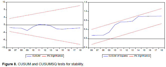
Stability test for money demand function in Turkey
The CUSUM and CUSUMSQ tests were performed to detect whether the coefficients of the money demand function were structurally stable with the null hypothesis of stable parameters. Figure 8, in which the blue lines are within the red line boundaries, implies that money demand function in Turkey is stable. This finding is similar to that of Saatcioglu and Korap (2005) in the study of Turkish broad money demand over the period 1987Q1 – 2004Q2 with quarterly data. However, in the analysis of money demand function in Turkey, Oscalik (2014) explains that while CUSUM test indicates stable money demand function, the CUSUMSQ test results in instability of money demand function. In the study conducted during the inflation target on money demand and its determinants in Turkey over the period 2002:Q1 – 2013:Q2, Tumturk (2017) also finds unstable relationship between money demand and its determinants with CUSUM test. The findings of their unstable money demand function might be attributed to the global financial crisis of 2008. However, the probability of this global-crisis impact is insignificant when a wide range of data period (1987 to 2018) is considered to investigate the stability of money demand function in Turkey.