ABSTRACT
The no-tillage technique has been expanding in the Brazilian Cerrado (savanna), but due to the rapid decomposition of residues and few options for profitable rotation crops, soil compaction can be a problem, seriously reducing water availability to plants. Determination of the least limiting water range (LLWR) is a sensitive method to assess the current soil compaction state, although it is operationally and economically beyond the reach of most farmers. Therefore, the aim of this study was to determine the LLWR of a highly loamy typic Oxisol (dystrophic red Latosol) and to evaluate the possibility of estimating it by using the relative bulk density (RBD), determined based on the soil compaction curve, which in comparison is a relatively fast and inexpensive method. The results showed that RBD was strongly correlated with LLWR, with coefficient of determination between 0.69 and 0.95, besides having low mean standard estimation error of at most 0.016 m3 m-3 (P < 0.0001), making measurement of the RBD satisfactory, to estimate the LLWR. Besides this, the RBD values corresponding to BDcritical, that is, when LLWR = 0, were very near the RBD value (≈ 0.90), taken as the upper limit of physical quality for adequate plant growth. Therefore, because of the high cost and laboratory time necessary to determine the LLWR for each type of soil, a viable alternative is to use the reference value or maximum acceptable RBD limit value of 0.90 for management of soil compaction, obtained through geostatistical analyses, to ascertain the variability in the cultivated areas where RBD ≥ 0.90. In short, it is technically and economically feasible to estimate the LLWR based on the RBD.
Key words: Soil compaction curve, proctor normal test without sample reuse, no-till farming in Mato Grosso, Midwest region of Brazil.
Farmers in the Brazilian Cerrado biome have widely adopted no-tillage techniques, mainly involving rotation of soybeans and corn, along with precision farming methods to define the use of inputs, instead of conventional management practices, which in the 1990s caused various problems associated with soil erosion and subsurface compaction (Altmann, 2010). However, no-till farming in the Cerrado region still faces problems of adaptation due to the rapid decomposition of residues and few economically feasible alternatives for rotation crops. These factors hinder control of surface compaction, one of the main obstacles to water availability to plants (Nawaz et al., 2013).
Several studies have described determination of the “least limiting water range” (LLWR) as a method that is sensitive and closely representative of the structural soil quality and the degree of soil compaction. This is important because to maximize crop yields, the water in the soil must be maintained at optimal levels (Collares et al., 2006; Moreira et al., 2014; Ramos et al., 2015). Furthermore, this method enables estimating the critical bulk density value (BDcritical), when the LLWR = 0, and hypothetically using it to monitor the physical soil quality (Betioli et al., 2012; Moreira et al., 2014; Safadousta et al., 2014).
However, routine use of LLWR measurement is not yet possible in Brazil, mainly for large farms and/or those employing precision agricultural techniques, where it is necessary to take a large number of samples to enable specific local correction of compaction. More important than the cost and time for sampling is the relative lack of laboratories equipped with the necessary infrastructure for testing samples. The few technically qualified laboratories that exist are either associated with universities, where research is the priority, or are privately run, with high cost for determining water retention curves, making it economically unfeasible for most farmers. This situation is unlikely to improve in the short or even medium term. Therefore, a satisfactory alternative can be the use of simpler methods to obtain one-time measures for each soil type and management method, having strong correlation with the least limiting water range. This will enable using the values obtained as references to estimate the LLWR to a sufficient degree of accuracy.
One of the laboratory techniques derived from geotechnical engineering used to reproduce compaction conditions for civil construction projects and farming operations is the Proctor test (normal or modified). It can determine the soil compaction curve quickly and inexpensively. For agronomic purposes, the importance of the compaction curve is related to determining the optimal compaction moisture, which is fast and at low cost. This allows inferring whether the soil moisture is too high for traffic of heavy machinery, because when this is the case, the bulk density and compaction can rise to unacceptable levels. The configuration of the compaction curve depends on, among other factors, the granulometry and organic carbon content. For agricultural purposes, it is recommended to determine the curve without reuse of soil samples (Ramos et al., 2013).
Therefore, because the relative bulk density, measured by the ratio between actual and maximum density through fitting, soil compaction curves can be useful to characterize compaction and the response of crops to different soil types (Hakansson and Lipiec, 2000; Suzuki et al., 2007). It was hypothesized that the LLWR can be estimated by using the relative bulk density, which can be measured quickly and inexpensively, to accelerate the mapping of compaction in agricultural areas in the Cerrado biome. To test this hypothesis, the ability to estimate the LLWR was assessed by correlation with the relative bulk density, using a highly loamy typic Oxisol (dystrophic red Latosol) under no-tillage management for 10 years.
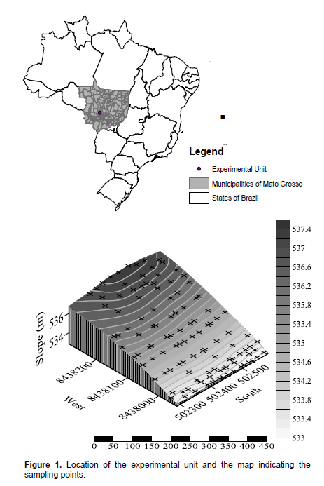
The study was carried out in the municipality of Diamantino (Mato Grosso State), located at 14° 07’ 40” S latitude and 56° 58’ 39” W longitude, at an altitude of 539 m. The region’s climate is Aw by the Köppen classification, with well defined seasons (dry from May to September and rainy from October to April). The average annual rainfall is 1816.9 mm, with maximum average temperature of 25.5°C and minimum of 16.2°C. The soil in the experimental field is classified as typic Oxisol (dystrophic red Latosol), moderate “A” horizon, with very loamy texture, in the semideciduous tropical forest phase, with flat relief (Santos et al., 2013). This soil class was chosen because it is the most representative of the State of Mato Grosso, Brazil.
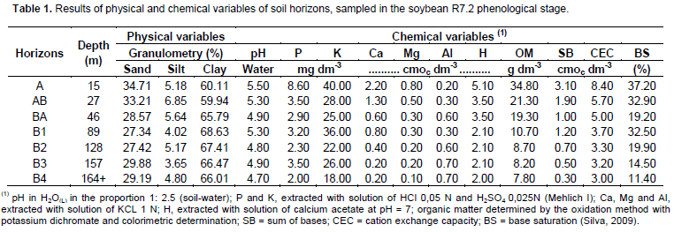
The area was cleared in 1987 and rice was planted (1987 to 88 crop), after which soybeans and corn were rotated until the 1999 to 2000 seasons, with harrowing to a depth of 0.20 m every three years and banding fertilization. Cotton was then grown from 2000 to 01 and 2003 to 04, after which soybeans and corn were again planted in succession from the 2004 to 05 and 2013 to 14 seasons, without harrowing but with broadcast application of lime and fertilizer. The present study was conducted during the 2013 to 14 growing season, specifically on the soybean crop (Glycine max L.), 7639 RR Monsoy cultivar, in an experimental plot measuring ≈ 12 hectares (300 by 405 m), part of a field covering 56 ha (Table 1). The plants were cultivated with row spacing of 0.45 m and an average of 15 plants per linear meter. The seeds were sown on October 23, 2013 and the plants were harvested on February 5, 2014.
Soil samples were collected at depths of 0 to 0.10, 0.10 to 0.20, 0.20 to 0.30 and 0.30 to 0.40 m, taking into account the root depth of plants. The sampling scheme was in irregular mesh, due to the varying level curves (recently restored), oriented between the rows, with 117 sampling points for each layer. These points were geo-referenced with maximum error, vertical and horizontal, of 5 mm, determined using a Topcon Hiper® Pro global positioning device (Figure 1).
One hundred and seventeen samples was collected from each layer to have the best set of statistical equations and to determine the spatial variability of soil relative bulk density, described later. The undeformed soil samples were collected when the plants were in the R7.2 stage, using an apparatus to dig and smooth the surface, after which the undeformed samples were obtained by inserting a Kopeck device with stainless steel cylinders (50 mm in diameter by 50 mm height) in the intermediate part of the layers. The samples were collected at the stadium R7.2 in order not to hinder the transit harvesting machinery, because it took seven days to collect all samples. 5 days to the end of the sample collection, the soybeans were harvested.
In the laboratory, the samples were saturated with distilled water and submitted to different matrix potentials, with 14 repetitions (to get better statistical adjustment): 2, 6, and 10 kPa, using a sandbox (Eijkelkamp Agrisearch Equipment model 08.01); and 33, 66, 100, 300 and 1500 kPa, using a Richards chambers (Soilmoisture Equipment Corp., model 1500F1).

After the samples at each potential reached the water balance point, they were weighed and then transferred to an electronic bench penetrometer with constant penetration speed of 10 mm min-1 (0.167 mm s-1), with a load cell having nominal capacity of 196.13 N (20 kgf), shaft with cone having diameter of 3.7407 mm and semiangle of 30°. The device was connected to a computer to record the readings (Bianchini et al., 2013). Then the samples were dried at 105°C for 48 h to calculate the bulk density (Donagema et al., 2011). These data were used to fit the water retention curve (WRC) and the mechanical penetration resistance (MPR) for each layer evaluated. The WRC was determined according to Moreira et al. (2014), using Equation 1:
Where: θ = soil water content (m3 m-3); Ψ = soil water potential (kPa); and BD = bulk density (Mg m-3), with a, b and c being the estimated coefficients.
In turn, the MPR was expressed as the ratio between θ and BD, according to Moreira et al. (2014), applying Equation 2:
where: MPR = the mechanical penetration resistance (MPa); and d, e and f are the estimated coefficients. The curves from equations 1 and 2 were fitted using a script programmed in the R Development Core Team software, version 3.0.1.
By ranking the bulk density values in increasing order, the upper limit of the LLWR was defined as the water content value related to the field capacity at water stress of 10 kPa (Silva et al., 1994), or by the aeration porosity of 10% (Silva et al., 1994), according to Equation 3:
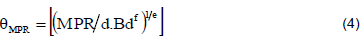
Where: AP = soil aeration porosity (m3 m-3); BD = bulk density (Mg m-3) (Donagema et al., 2011); and PD = average particle density: 2.40 (0 to 0.10), 2.50 (0.10 to 0.20), 2.55 (0.20 to 0.30) and 2.68 Mg m-3 (0.30 to 0.40 m). In turn, the lower limit of the LLWR was defined as the moisture corresponding to the permanent wilting point based on water stress of 1500 kPa (Silva et al., 1994), or mechanical penetration resistance at a limiting value of 2.0 MPa (Silva et al., 1994), using Equation 2 rewritten in the form of Equation 4:

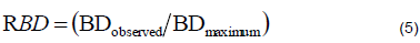
To determine the soil compaction curve without sample reuse, the dug transversal trenches was used in the experimental plot and approximately 80 kg of soil was collected, with a preservation of the natural structure of the clumps for each layer evaluated. The samples were placed in polyethylene boxes and taken to the laboratory, and the techniques described in Ramos et al. (2013) was applied. Based on the data pairs of the gravimetric moisture (GM) and bulk density (BD) the model were adjusted, that is by regression, applying a polynomial quadratic equation (BD = y0+aGM – bGM2), where y0, b and c are the estimated coefficients. The relative bulk density (RBD) was determined according to Klein (2006) by Equation 5:

Where: BDobserved = bulk density at the sampling point (Mg m-3); and BD = maximum bulk density for each layer evaluated (because of a possible influence of the vertical variability of soil organic matter, shown in Table 1), obtained by calculating the maximum point for each compaction curve (yvertex, Mg m-3 = - (b2 – 4ac)/4a).
The bulk density data were normally distributed according to the Shapiro-Wilk test (P > 0.05), with coefficients of variation lower than 5.83%. The accuracy of the linear regressions was evaluated by the F-test (α = 0.05) and the coefficient of determination (R²), using the SigmaPlot 12.5 software. Analysis and modeling of the spatial structure of the relative bulk density was carried out by the ordinary Kriging method, in 2 × 2 m squares (Yamamoto and Landin, 2013). The isotropic semivariograms were fitted using the Gamma Design GS+TM version 10.0 software from Geostatistics for the Environmental Sciences.
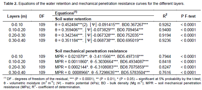
The results of fitting the data on water retention and penetration resistance explained more than 90% of the soil volumetric moisture and 76% of the penetration resistance at the 5% probability level (α = 0.05) (Table 2). Besides this, the coefficients of the models, besides differing from zero based on the t-test, had the expected signs according to the theory, that is, the volume of water retained in the soil samples was inversely proportional to the reduction of the matrix potential and directly proportional to the increase in bulk density, while the mechanical penetration resistance was inversely proportional to rising water content and directly proportional to increasing bulk density. These results are consistent with other studies (Collares et al., 2006; Moreira et al., 2014; Ramos et al., 2015).
With increasing bulk density, the volumetric water content values at which the mechanical penetration resistance reached the critical value (θPR) occurred above all the water content values equivalent to the permanent wilting point limit (θPWP), causing a sharper reduction of the LLWR (Figure 2A to D). This stronger influence of θPR on the configuration of the LLWR has been reported for different soil classes, when native environments are converted to farming and livestock breeding uses (Betioli et al., 2012; Moreira et al., 2014;
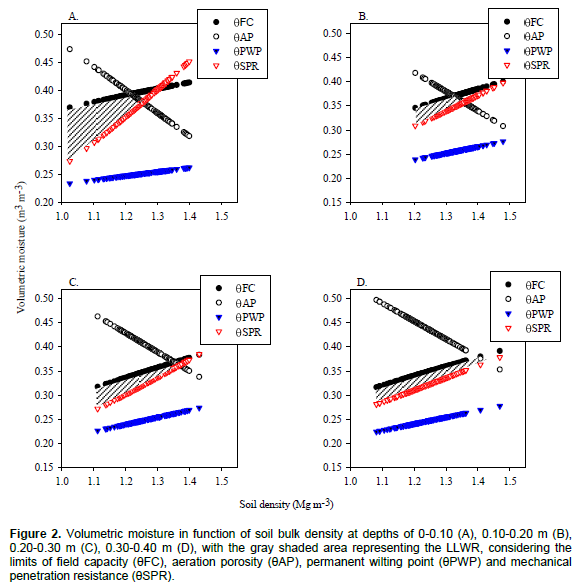
The critical bulk density values found for the depths of 0 to 0.10, 0.10 to 0.20, 0.20 to 0.30 and 0.30 to 0.40 m were, respectively, 1.257, 1.360, 1.374 and 1.468 Mg m-3 (Figure 2). BDcritical was attained with smaller bulk density values in the surface layer, although a compensating effect occurred of smaller bulk density values and increased amplitude of the LLWR (Figure 2A). According to Altmann (2010), this result can be associated with the direct and indirect benefits from the longer time to accumulate organic matter when the soil is left fallow. The accumulation possibly improved the soil structure, culminating in larger macropores in the soil under no-till farming, because based on compound analysis of the 117 sampling points, we found the following average organic matter values: 38.90 g dm-3 (0 to 0.10 m); 35.80 g dm-3 (0.10 to 0.20 m); 26.3 g dm-3 (0.20 to 0.30 m); and 23.4 g dm-3 (0.30 to 0.40 m). Furthermore, although the layer thickness were different, it was also possible to observe the decrease of soil organic matter in depth (Table 1).
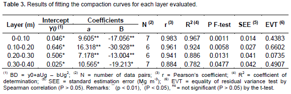
With respect to the soil compaction curves, the statistical models were satisfactory because the results were significant (P < 0.05), with standard estimation error of at most 0.042 Mg m-3 and equality of residual variance (P > 0.05). Besides this, the bulk density values obtained with compaction of the deformed samples in the cylinder, according to the Proctor normal test, presented satisfactory explanatory power, because the coefficient of determination was higher than 78% (Table 3). The reason this was not higher might be that the soil in the present study is very plastic and sticky, as reported by Santos et al. (2013), which hindered compaction of the samples in the cylinder.
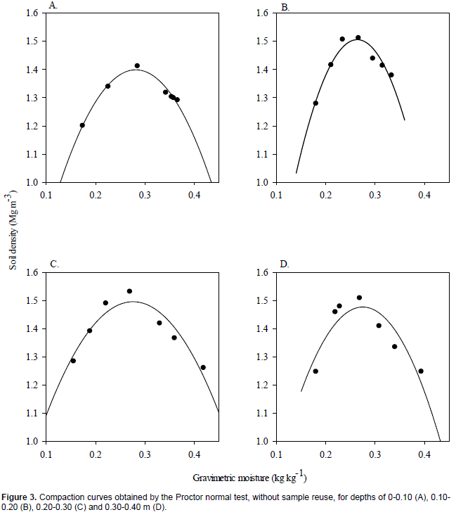
The optimal compaction moisture (Moptimal) and corresponding maximum bulk density values for each layer evaluated were 0.281 kg kg-1 and 1.399 Mg m-3 (0 to 0.10 m), 0.263 kg kg-1 and 1.506 Mg m-3 (0.10 to 0.20 m), 0.275 kg kg-1 and 1.496 Mg m-3 (0.20 to 0.30 m) and 0.274 kg kg-1 and 1.477 Mg m-3 (0.30 to 0.40 m) (Figure 3). The Moptimal value indicates where traffic of machinery should be avoided, because the increase in water content makes the soil easier to compact. In contrast, according to Ramos et al. (2013), reduction in the water content can cause stronger coherence of the particles, making the soil less susceptible to compaction.
Based on this, it was found that the gravimetric water contents that resulted in the highest compaction density in each soil layer were approximately 5% below the volumetric moisture equivalent to the field capacity (θCC = 10 kPa) for each layer, that is, by substituting the values in the water retention equations (Table 2), the respective values of BDcritical (Figure 2) produced corrected values for gravimetric moisture of 0.257, 0.277, 0.271 and 0.266 kg kg-1 for layers 0 to 0.10, 0.10 to 0.20, 0.20 to 0.30 and 0.30 to 0.40 m, respectively (Figure 3). Therefore, the water content values near field capacity indicate the maximum susceptibility of the soil to compaction. This means that determining the water content in the soil before use of heavy machinery in the field is important, because small variations in water content can cause substantial increases in bulk density.
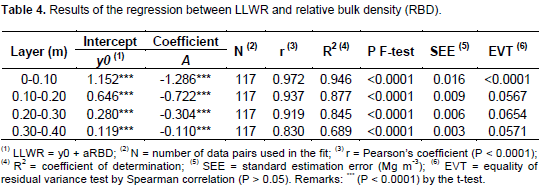
The relative bulk density (RBD) values presented strong correlation with the LLWR, higher than 0.80 by the Pearson test. Besides this, the ability of the RBD value to explain the LLWR was satisfactory, with a coefficient of determination varying from 68 to 94%. Furthermore, the adjustments for all layers were highly significant by the F-test, with intercept and coefficient other than zero by the t-test, besides small standard estimation error of at most 0.017 m3 m-3 (Table 4).
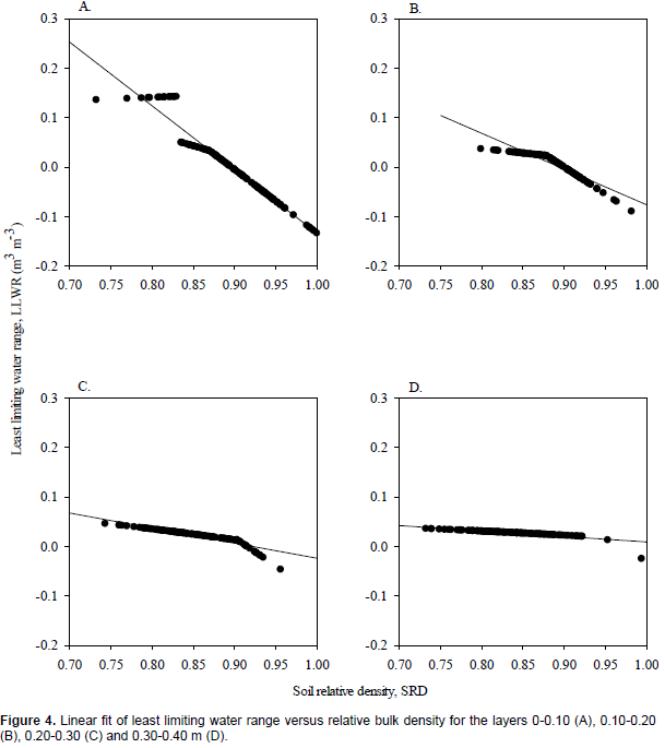
However, the occurrence of independent residual error appeared to depend on something not controllable, namely the intersection of the curves that configure the LLWR. In other words, when the data pairs are discontinuous (Figure 4A), there appears to be a higher probability that the variance test will not indicate residual equality.

The ratios between RBD and BDcritical for the four soil layers were 0.913 (0 to 0.10 m, Figure 4A), 0.903 (0.10 to 0.20 m, Figure 4B), 0.918 (0.20 to 0.30 m, Figure 4C) and 0.953 (0.30 to 0.40 m, Figure 4D). According to the literature, the interval of values considered ideal for optimal soybean crop yield vary between 0.82 and 0.91 (Hakansson and Lipiec, 2000; Beutler et al., 2005; Suzuki et al., 2007; Betioli et al., 2012). Therefore, the values of RBD = BDcritical (LLWR = 0) found in this study (Figure 4) were approximately in line with the ideal maximum limit for plant development found in the literature. Therefore, it would be technically practical to use a reference value of RBD = 0.90 to monitor the compaction of any agricultural soil, since RBD values greater than 0.90 are not ideal for plant growth. This would make it unnecessary to determine the LLWR for each type of soil, because it would be sufficient to estimate the RBD value and use 0.90 as the upper threshold. However, it is important to standardize the method for determining the compaction curve to obtain the maximum soil density, preferably without reuse of samples for considering the soil structure, as urged by Ramos et al. (2013).

In this study, the proportion of the BD or RBD values ≥ BDcritical (LLWR = 0) for the depths of 0.20 to 0.30 m and 0.30 to 0.40 m were, respectively, only 8 and 2% of the 117 samples collected. In contrast, for the 0 to 0.10 and 0.10 to 0.20 m layers, 50 and 34%, and of the values were above the BDcritical. Since soil management typically occurs in the topmost layer, and the best estimates of the LLWR by using the RBD were provided by the 0 to 0.10 and 0.10 to 0.20 m layers, special attention should be paid to these two layers. Based on these findings, since the LLWR was satisfactorily estimated by the RBD, our hypothesis can be accepted, meaning that the variability in space of the RBD can help support decisions on actions to prevent soil compaction, making it a useful technique for farmers using precision techniques for localized correction of soil compaction. The results also indicate that exponential isotropic semivariograms explained from 77 to 91% of the RBD, with lower range value in the 0.20 to 0.30 m layer, showing smaller spatial homogeneity. Nevertheless, all the layers evaluated presented high spatial dependence, demonstrating the data are not random, based on the value of C/Co + C near 1.0 (Table 5).
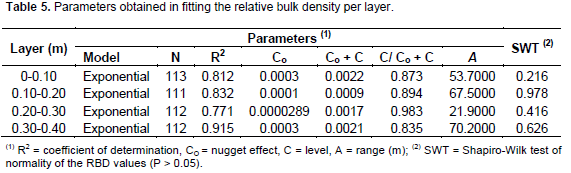

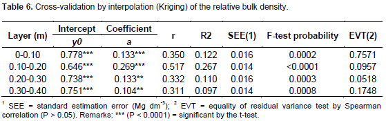
Next the cross-validation of the observed and estimated data was analyzed by Kriging. The majority of published works do not provide the result of this validation. Although the coefficients of determination of the fitted semivariograms were high, that is, greater than 0.771 (Table 5), with the cross-validation test we obtained weak explanation (R2 < 0.30) and moderate linearity (0.30 < r < 0.50), although with standard estimation error of at most 0.016 for the RBD value. Additionally, the models’ results were significant for the layers evaluated (P < 0.05 by the F-test) (Table 6). Therefore, it is essential to analyze the semivariogram along with the cross-validation results, because it is possible for the coefficient of determination to be high in the semivariogram, but with error probability greater than 5% (α = 0.05) by the F-test in the cross-validation, thus invalidating the fitted semivariogram.
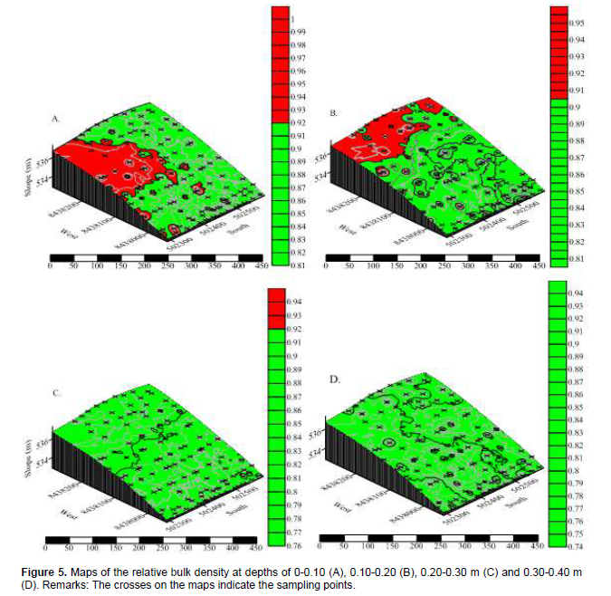
In this study, since the linear regressions were significant at probability of 5% (α = 0.05) by the F-test, the models were accepted. Therefore, we generated the maps of spatial variability of the RBD values for the layers evaluated based on data interpolation by Kriging at regular intervals of 1.0 by 1.0 m, considering the limits of the RBD values (Figure 4), that is, when LLWR = 0 (Figure 5).

It can be seen that the area with RBD values ≥ 0.913 was greater in the surface layer and concentrated to the west, and in the 0.10 to 0.20 m layer to the north. In the 0.20 to 0.30 m layer, although the legend shows the presence of RBD ≥ 0.918, the locations of these values coincide with the sampling points. This means a sub-area for specific management was not created, because of the low number of RBD values ≥ 0.918, but if RBD values < 0.918 were chosen, sub-areas in red would appear, that is, a cutoff limit on the map. For this reason, it is important to define this limit to know whether or not it is financially sound to carry out localized soil compaction correction.
The number of samples collected in this study, 117, to cover a small area of approximately 12 ha, was in line with the sampling density recommended by Yamamoto and Landin (2013), of at least 100 observations for a first study in any area. In the deepest layer (0.30 to 0.40 m) we did not observe RBD values > 0.953, because although this occurred according to Figure 4, when the LLWR = 0, it was necessary to remove a small percentage of the data (under 5%) to improve the fit of the semivariogram, a valid procedure according to Yamamoto and Landin (2013). In light of this, for future studies using the RBD to monitor the variability of compaction, we recommend distance between sampling points of between 21 and 70 m (Table 5), preferably arranged in a regular grid, which was not possible here. According to Yamamoto and Landin (2013), a regular arrangement of sampling points can improve the semivariogram fit, the cross-validation and the quality of the data interpolation, and consequently the configuration of the final map.
1. The relative bulk density (RBD) was strongly correlated with the least limiting water range (LLWR), so the ability of the RDB to explain the LLWR was satisfactory, presenting a coefficient of determination between 0.69 and 0.95, besides having a low standard estimation error, of at most 0.016 m3 m-3, which corresponds to only 3.1% to the total soil porosity, and a highly significant fit (P < 0.0001).
2. Besides this, the RBD values found corresponding to BDcritical, that is, when LLWR = 0, were very near RBD ≈ 0.90, taken as the upper limit for physical quality for adequate plant growth reported in the literature. Therefore, because of the high cost and laboratory time necessary to determine the LLWR for each type of soil, a viable alternative is to use the reference value or maximum acceptable RBD limit of 0.90 for management of soil compaction, obtained through geostatistical analysis, to ascertain the variability in the cultivated areas where RBD ≥ 0.90. In short, it is technically and economically feasible to estimate the LLWR based on the RBD, although it is important to standardize the method for determining the compaction curve to obtain the maximum soil density, preferably without reuse of samples to consider the soil structure.
The authors have not declared any conflict of interest
REFERENCES
|
Altmann N (2010). Plantio Direto no Cerrado: 25 anos acreditando no Sistema. Aldeia Norte Editora: Passo Fundo, RS, Brasil, 568 p.
|
|
|
|
Betioli JE, Moreira WH, Tormena CA, Ferreira CJB, Silva AP, Giarola NFB (2012). Intervalo hídrico ótimo e grau de compactação de um Latossolo Vermelho após 30 anos sob no-tlll farming. Rev. Bras. Ciênc. Solo 36(3):971-982.
Crossref
|
|
|
|
|
Beutler AN, Centurion JF, Roque CG, Ferraz MV (2005). Densidade relativa optimal de latossolos vermelhos para a produtividade de soja. Rev. Bras. Ciênc. Solo 29(6):843-849.
Crossref
|
|
|
|
|
Bianchini A, Roque MW, Rosa RP (2013). Development of an automated bench top electronic penetrometer. Eng. Agríc. 33(6):1191-1199.
Crossref
|
|
|
|
|
Collares GL, Reinert DJ, Reichert JM, Kaiser DR (2006). Qualidade física do solo na produtividade da cultura do feijoeiro num Argissolo. Pesq. Agropec. Bras. 41(11):1663-1674.
Crossref
|
|
|
|
|
Donagema GK, Campos DVB, Calderano SB, Teixeira WG, Viana JHM (Org.) (2011). Manual de Métodos de Análise de Solo. 2nd ed. Rio de Janeiro: Embrapa Solos, P. 230.
|
|
|
|
|
Hakansson I, Lipiec J (2000). A review of the usefulness of relative bulk density values in studies of soil structure and compaction. Soil Till. Res. 53(2):71-85.
Crossref
|
|
|
|
|
Klein VA (2006). Densidade relativa - um indicador da qualidade física de um latossolo vermelho. Rev. Ciênc. Agrovet. 5(1):26-32.
|
|
|
|
|
Moreira FR, Dechen SCF, Silva AP, Figueiredo GC, De Maria IC, Pessoni PT (2014). Intervalo hídrico ótimo em um Latossolo Vermelho cultivado em sistema semeadura direta por 25 anos. Rev. Bras. Ciênc. Solo 38(1):118-127.
Crossref
|
|
|
|
|
Nawaz MF, Bourrié G, Trolard F (2013). Soil compaction impact and modelling. A review. Agron. Sustain. Dev. 33(2):291-309.
Crossref
|
|
|
|
|
Ramos FT, Maia JC, Roque MW, Azevedo EC, Campelo Júnior JH, Weber OLS, Bianchini A (2015). Correlation of the least limiting water range with soil physical attributes, nutrient levels and soybean yield. Afr. J. Agric. Res. 10(21):2240-2247.
|
|
|
|
|
Ramos FT, Ramos DT, Maia JCS, Serafim ME, Azevedo EC, Roque MW (2013). Curvas de compactação de um Latossolo Vermelho-Amarelo: Com e sem reuso de amostras. Rev. Bras. Eng. Agríc. Ambient. 17(2):129-136.
Crossref
|
|
|
|
|
Safadousta A, Feizeea P, Mahboubib AA, Gharabaghib B, Mosaddeghic M R, Ahrensd B (2014). Least limiting water range as affected by soil texture and cropping system. Agric. Water Manage. 136(1):34-41.
Crossref
|
|
|
|
|
Santos HG, Jacomine PKT, Anjos LHC, Oliveira VA, Lumbreras JF, Coelho MR, Almeida JA, Cunha TJF, Oliveira JB (2013). Sistema Brasileira de classificação do solo. 3rd ed. Brasília: Embrapa Solos, 353 p.
|
|
|
|
|
Santos RD, Lemos RD, Santos HG, Ker JC, Anjos LHC, Shimizu SH (2013). Manual de Descrição e Coleta de Solo no Campo. 6th ed. Sociedade Brasileira de Ciência do solo, Viçosa, MG, Brasil, 2013. 100 p.
|
|
|
|
|
Silva AP, Kay BD, Perfect E (1994). Characterization of the Least Limiting Water Range. Soil Sci. Am. J. 58:1775-1781.
Crossref
|
|
|
|
|
Suzuki LEAS, Reichert JM, Reinert DJ, Lima CLR (2007). Grau de compactação, propriedades físicas e rendimento de culturas em Latossolo e Argissolo. Pesq. Agropec. Bras. 42(8):1159-1167.
Crossref
|
|
|
|
|
Yamamoto JK, Landim PMB (2013). Geoestatística: Conceitos e aplicações. Oficina de Textos: São Paulo, SP, Brasil, 215 p.
|
|