ABSTRACT
This work aims to study the integration of papaya market, price transmission and price causality patterns with the help of Johansen co-integration test, vector error correction model and Granger causality test using 13 years average monthly prices of papaya. Johansen co-integration tests indicate that four papaya markets significantly co-integrated with each other. Vector error correction (VEC) model test indicates that speed of papaya price adjustment for Arbaminch market was statistically significant at 1% level and the fastest compared to other payaya price adjustment. Its equilibrium price was stable. Whereas, speed of price adjustment for Adama market was insignificant and the slowest as compared to other market prices; its equilibrium was unstable because price change was away from equilibrium price. This implies that there was asymmetric information. The Granger causality test indicates that Arbamnch papaya price had bidirectional relationships with Merkato and Shashemenie markets. Concerned bodies should work on asymmetric information to address slow price adjustment between various papaya markets.
Key words: Market integration, papaya, vector error correction model, Granger causality.
Spatial market integration strengthens successful trade between food-deficit and food-surplus areas. This leads to specialization and economic growth. Moreover, market integration has a great contribution to food security and economic growth. It also improves producers’ and consumers’ social welfare, particularly in a diverse and highly vulnerable country such as Ethiopia. It accelerates effective price transmission between markets with the help of market reforms (Golettie and Babu, 1994). On the contrary, poor food price integration has unfavorable effects on social welfare of producers and consumers (Goletti et al., 1995). Poor market integration could also reflect the existence of imprecise price information, presence of either state policies or infrastructural and institutional problems that influence producers’ market decisions and the efficient flow of goods between markets. The marketable surplus generated by farmers could then result in depressed farm prices and diminishing income (Tahir and Riaz, 1997).
Market integration is expected to ensure a more rapid and effective price adjustment between markets with the help of market reforms (Golettie and Babu, 1994). Thus, government has paid attention to agricultural market integration in developing countries (Abdulai, 2000; Van Campenhout, 2006; Amikuzuno, 2009).
Price is a basic means to tie different stages of a market chain. Price signals could be a good evidence of market segmentation or potential manipulation, distortion of price information which causes inefficient allocation of resources. These situations do not attract farmers to produce marketable surplus because of low price which causes low income (Tahir and Riaz, 1997). Price shocks are passed on from one stage to next stage of market chain and the extent of adjustment to such shocks constitutes important factors reflecting the actions of market participants at different market levels. The speed of price adjustment greatly relies upon the kind of products. Fruit markets have high probability to adjust price rapidly. On the contrary, in some level processed products and non-perishable products have low chance to adjust price. It is deemed that price adjustment between various stages in the market chain is not symmetric (Reziti and Panagopoulos, 2008). This means that positive and negative price shocks are not transmitted in the same way.
Moreover, in developing countries poor infrastructure and transport services results in large marketing margins due to high costs of delivering traded commodities. High transfer costs hinder the transmission of price signals, and they may prevent or discourage goods arbitrage (Sexton et al., 1991). Investigation of market integration is useful to understand the function of market; design and adopt most suitable agricultural price stabilization policies (Seneshaw, 2013).
Thus, it is crucial to conduct this research because there is no empirical evidence about spatial market integration and its price transmission in Ethiopian papaya prices. Information on market integration is thus useful in making agricultural policies, including policies and strategies for price stabilization, price risk management and food security. Moreover, this study helps to come up with the latest, accurate, reliable, and prompt information about market integration of papaya prices across markets and speed of price transmission in Ethiopia. This result is also useful to generate information and fill knowledge gaps in the spatial papaya market integration and its price transmission.
Therefore, this study examines the degree of spatial domestic papaya market integration; its price transmission; and causality patterns using Johansen co-integration test, vector error correction model and Granger causality test.
Market integration can be classified into three: (1) vertical market integration which includes different stages in marketing and processing channels; (2) spatial integration which relates to spatially distinct markets; and (3) inter-temporal market integration which refers to arbitrage across periods of time (Barret as cited by Uchezuba, 2005). This study focuses on spatial integration of papaya prices among a number of markets in Ethiopia.
The spatial arbitrage condition is that market integration leads itself to a co-integration interpretation which is measured co-integration tests (Fackler and Goodwin, 2002). If two spatially separated price series are co-integrated, then there is a tendency for them to co-move in the long run according to a positive linear relationship. In the short run, the prices may drift apart, as shocks in one market may not be instantaneously transmitted to other markets due to delays in transport or information; however, arbitration opportunities ensure that these divergences from the underlying long run (equilibrium) relationship are transitory and not permanent.
The analysis of spatial market integration attempts to address three main questions about the nature of the price transmission process among spatially separated markets; such as causality patterns, dynamic interactions, or long-run equilibrium. Co-integration analysis is only concerned with the existence of long run equilibrium between markets, and cannot answer questions pertaining to the price adjustment process over time. But, the vector error correction (VEC) addresses question of the price adjustment process over time.
However, various authors postulated and applied various analysis methods to assess market integration. Also, Meyer and Von Cramon-Taubadel (2002) pointed out that there is still no unified approach to evaluate market integration. Market integration can be measured in different ways, including the movement of goods. Previously, price correlation coefficients were used to investigate whether or not markets were linked by price changes (Timmer, 1987; Dadi et al., 1992). However, price correlation coefficients may mislead the results due to the presence of trends (non-stationary data) in the data (Wyeth, 1992). Regression analysis has also been used to analyze integration (Alexander and Wyeth, 1994). This practice was modified using price variables in their first difference form, but this caused the loss of long-run information. Co-integration, on the other hand, allows a way of dealing with time series data that avoids spurious results, thus enhancing the validity of research findings. Johansen’s approach to co-integration is now used widely to test the level of integration among markets. Several authors applied threshold autoregressive models to deal with asymmetric price transmission in agricultural marketing. Unit root test and Co-integration test do not have power to check the prevalence of asymmetric adjustment because they assume symmetric and linear adjustment. So, Enders and Siklos (2001) suggest an extension to standard ECM which appears in the literature as threshold autoregressive (TAR) model. However, the TAR models have calculation challenges and impose ex-ante non-theoretical restrictions. Additionally, TAR models are suggested to check the existence of non-linear transaction costs and price bands. Therefore, Johansen’s approach to co-integration, VECM and Granger causality are proposed for this study to investigate market integration, price adjustment and causality patterns of papaya markets in Ethiopia respectively.
Source of data
The study aimed to analyze the degree of market integration and price adjustment of papaya markets among three regions in Ethiopia. Average monthly retailer prices with 156 total observations were gathered from CSA data bases from September 2002 to September 2014. Five markets for price of papaya were selected for this study based on the availability of data, surplus and deficit markets.
Methods of analysis
The time series data are stationarity when conditional mean, variance, and auto-covariance are constant over time. If x and y have unit root, the standard t-test is invalid, which leads to equation 1 to come up with a spurious regression.
Time series is non-stationarity when conditional mean, variance and auto-correlation are not constant over time. If they are not constant over time, then the series is said to be a non-stationary process (i.e. a random walk/has unit root). Differencing a series using differencing operations produces other sets of observations such as the first-differenced values, the second-differenced values and so on.
If a series is stationary without any differencing it is designated as I (0), or integrated of order 0. On the other hand, a series that has stationary first differences is designated I (1), or integrated of order one (1). Augmented Dickey-Fuller test has been suggested by Dickey and Fuller, (1979) while the Phillips-Perron test recommended by Phillips and Perron (1988) has been used to test the stationarity of the variables. The price variables have been tested for unit roots by the Augmented Dickey-Fuller (ADF) test with different specifications, with trend and constant:

Where α, β and

g are coefficients, r is the number of lagged variables specified and
et is the random term to be estimated and tested. This test statistic is probably the best-known and most widely used unit root test. It is a one-sided test whose null hypothesis is β=0 versus the alternative β
< 0 (and hence large negative values of the test statistic lead to the rejection of the null). Under the null, y
t must be differenced at least once to achieve stationarity; under the alternative, y
t is already stationary and no differencing is required.
If all the variables are stationary, the VAR can be used; OLS can also be used to estimate each equation and standard statistical methods can be employed. If some of the original variables have unit roots and are not co-integrated, then the ones with unit roots should be differenced and the resulting stationary variables should be used in the VAR. If the variables have unit roots and are co-integrated, the vector error correction model should be used.
Johansen and Juselius cointegration test
Johansen and Juselius (1990) suggest Maximum Eigenvalue test and the Trace test to determine the number of co-integration vectors. The Maximum Eigenvalue statistic tests the null hypothesis of r co-integrating relations against the alternative of r+1 co-integrating relations for r = 0, 1, 2…k-1. This test statistics are computed as:
Where l
is the estimated Maximum Eigenvalue and T stands for the sample size. The trace test conducts a joint test whereas the maximum Eigenvalue test carryout separate tests for the individual eigenvalues. Trace statistics examines the null hypothesis of r co-integrating relations against the alternative of n co-integrating relations, where n is the number of variables in the system for r = 0, 1, 2…k-1. It is formulated as follows:
The results of trace test are preferred while Trace and Maximum Eigenvalue statistics come up with different results in some case (Alexander, 2001). If a long-term equilibrium relationship exists between time series data, price adjustment is conducted to evaluate the short run properties of the co-integrated series with the help of VECM. VECM is not needed to carry out, if time series data not co-integrate.
Vector error correction model (VECM)
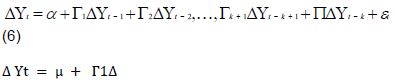
VECM can be applied to measure price adjustment. Adjustment of prices induced by deviations from the long-term equilibrium (ECT) is assumed to be a continuous and linear function of the magnitude of the deviation from long-term equilibrium. Thus, even very small deviations from the long-term equilibrium will always lead to an adjustment process in each market. If time series data are co-integrated this implies that there exists a long-term equilibrium relationship between them so VECM can be applied to evaluate the short run properties of the co-integrated series. If co-integration is not absent between series, VECM will no be longer required. So, Granger causality tests are directly applied to see causal relationship between variables. Given the following general specification of the VECM model which considered with VAR .
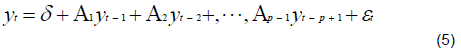
Where Yt is an (n x 1) vector of endogenous variables (prices), δ is an (n x 1) vector of parameters, y and yt-p are lagged values of prices; Ai represents (n x n) matrices of parameters, and εt is an (n x 1) vector of random variables. In this model, the price series for the five papaya markets were endogenous variables and as such no exogenous variable was used. To test the hypothesis of integration and co-integration in Equation 5, we transform it into its vector error correction form.
Where Yt =[P1t, P2t]', vector of endogenous variables, which are I(1), Δ Yt= Yt- Yt-1, a is a (2×1) vector of parameters, Г1,..., Гk+1 and π are (2×2) matrices of parameters, and εt is a (2×1) vector of white noise errors. Where π is of a reduced rank, that is r≤1, it can be decomposed into π =αβ' and when r=1, α= [α1, α2]' is the adjustment vector and β= [β1, β2]' is the co-integrating vector.
The existence of co-integration and error correction representation implies the existence of causality in at least one direction (Granger, 1988). However, co-integration itself is not useful to deduce about the direction of causation between series. Thus, Granger causality test is necessary. Granger causality test focuses on the presence of unidirectional causality linkages as an indication of some extent of integration (Gupta and Mueller, 1982). Bi-directional causality implies that both markets depend each other on market price information to set their price while unidirectional causality implies only one market uses other market price information to set its own price. Granger causality specification for co-integrated variables is written as:
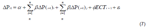
Where Δ is the difference operator, Pi1 and Pj2 are papaya prices; are white noise error terms, ECTt-1 is the error correction term derived from the long-run co-integrating relationship, while r is the optimal lag of the variables which are chosen with the help of Akaike criterion (AIC), Schwarz Bayesian criterion (BIC) and Hannan-Quinn criterion (HQC) (Hendry and Ericsson, 1991).
Stationarity test
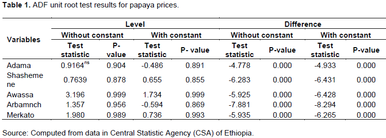
For co-integration analysis, it is important to test the unit roots with the help of the Augmented Dickey- Fuller (ADF) at the beginning to check whether modeled variables I (0) at levels and I (1) at first differences were stationary or non- stationary. The tests were applied to each variable over the period of 2001-2013 with and without constant at the variables level and at their first difference.
The result in Table 1 indicates that the null hypothesis of no unit roots for all the time series were rejected at their levels. On the other hand, the all variables were stationary and integrated of same order, that is, I (1) at their first difference for both with and without constant, which means unit roots in the first differences were rejected at 1%. Therefore, the results allow proceeding for co-integration tests for the testing of the long run equilibrium relationship.
Moreover, according to Mesike et al. (2010), any endeavor to determine the dynamic function of the variable in the level of the series based on results of the variables are I (1) and I (0) will be inappropriate and may lead to problems of spurious regression. The econometric results of the model cannot be used for prediction in the long-run in that level of series because it will not be ideal for policy making (Yusuf and Falusi, 1999).
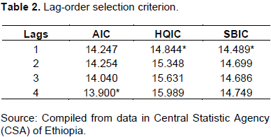
ADF test results enable researcher to conduct Johansen co-integration test which is suitable to see the existence of long-run relationships among variables because they fulfill the precondition for co-integration analysis. In this study, the optimal number of lag for VAR model was determined based on value of Akaike criterion (AIC), Schwarz Bayesian criterion (BIC) and Hannan-Quinn criterion (HQC).
The result in Table 2 shows that candidate of optimal lag of the AIC is lag 4; optimal lag of SBIC and HQIC is lag 1. As we can see in Table 2, there is more than one candidate of optimal lag exist, so the value of R2 from the VECM analysis was checked with lag 1 and lag 4. Based on the results of VECM analysis, lag 4 is found to be optimal lag for this model because it yields higher R2.
Johansen co-integration tests
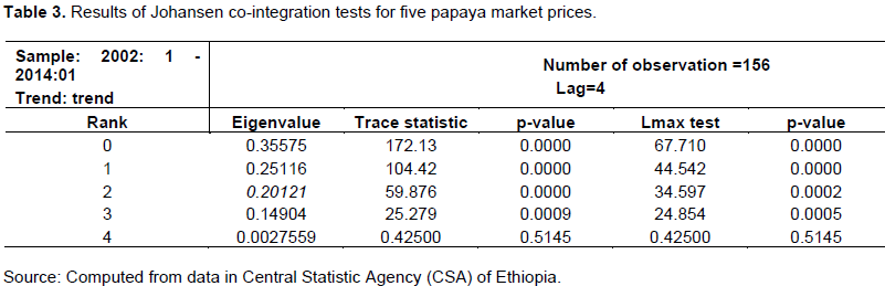
To state a co-integration model, Johansen’s testing procedure was followed. Each co-integrating equation has an intercept and a slope coefficient. The null hypotheses for the trace test are rejected at the 10% level of significance; we reject the null hypotheses that r=0 and r <1, but we failed to reject the null hypothesis that the co-integrating rank of the system is at most two.
Johansen’s trace and -max tests rejected first four hypotheses (r = 0 to 3) of no co-integrating vector at 1% level of significant; Johansen trace statistic rejected 0-3 hypotheses(r=0, r=1 r=2, r=3) at 1% level of significant. In other words, this trace test result rejected the null hypotheses because these four variables were co-integrated (Table 3). These results suggest that there are four long-run equilibrium relationships between the five price series.
Vector error correction model
The ADF test results approve that a VEC model is more pertinent than a vector autoregression model to distinguish the multivariate interactions among the three price series (Engle and Granger, 1987). That is, all price series data which have unit roots are more pertinently examined the existence of a number of long run co- integration vectors than a vector autoregression model.
The presence of co-integration between variables suggests a long term relationship among the variables under consideration. The coefficient of price adjustment with negative sign indicates a backward movement towards equilibrium; a positive sign indicates movement away from equilibrium. The coefficient should lie between 0 and 1, 0 suggesting no adjustment one time period later, 1 indicates full adjustment. The coefficients of the error correction term show the speed of convergence to the long run equilibrium as a result of shock of their own prices.
In this study, coefficient of dynamic adjustments that is obtained with the help of the VEC model analysis is used to estimate the speeds of price transmission. The results of the speeds of adjustment/adjustment vectors are displayed in Table 4. The speeds of adjustment for Arbamnch retail papaya price were statistically significant at 1% level. The speeds of adjustment for Adama and Merkato the retail price were not statistically significant. The estimate of the error correction coefficients for the selected papaya markets indicates that Shashemenie market was significant at 1% with a wrong sign (positive). This shows that any disequilibrium in the long run retailer price would be corrected in the short run; thus, the short run price movements along the long run equilibrium path may be unstable (Table 4). The coefficient of adjustment vector (α) for Awassa market has a wrong sign (positive) and significant at 1% level showing that the short run price movements along the long run equilibrium path may be unstable.
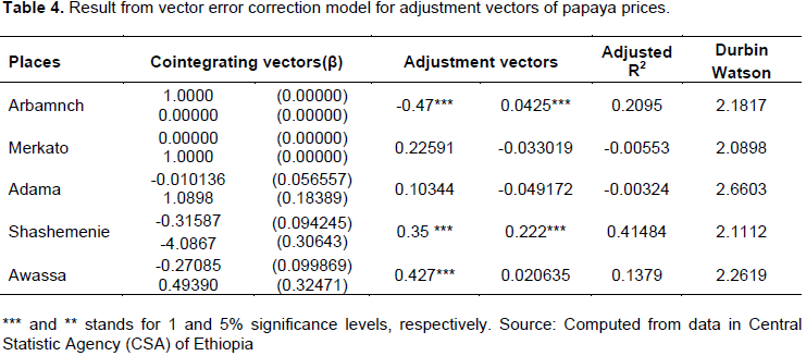
The speed of adjustment for Arbamnch papaya price has the expected negative sign because of the overreaction of prices in the short run in response to an exogenous shock. The dynamic speed of adjustment for the Arbaminch price was higher (0.47), in absolute value, than other papaya market prices, an indication of asymmetric price transmission with respect to speed. This is an interesting result suggesting that with the safety shock, Arbamnch prices adjust more quickly and are more flexible than farm prices to restoration in the long-run equilibrium. This result is also important for policy makers and agribusinesses and has clear implications for the efficiency and equity of the Ethiopia papaya marketing system. It indicates that the speeds of price adjustment are not the same in different markets. Prices in the Arbamnch market adjust more quickly than prices at other market in response to the safety shock.
Even if we demonstrate market integration through co-integration, there could be disequilibrium in the short run, i.e., price adjustment across markets may not happen instantaneously. It may take some time for spatial price adjustments to occur. The error correction model takes into account the adjustment of short-run and long-run disequilibrium in markets and time to remove disequilibrium in each period. In terms of efficiency, prices are transmitted fully and completely given efficient market conditions. The fact that price dynamics differ might point to noncompetitive market conditions that can lead to market inefficiencies. It is important to note that our analysis cannot directly test for imperfect competition and does not explicitly address imperfect competition. Future research and modeling efforts are required to address this hypothesis directly and appropriately.
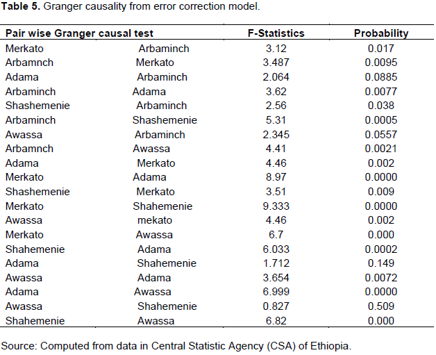
Granger causality tests
Granger causality was also estimated between pairs of papaya market prices. Granger causality means the direction of price formation between two markets and related spatial arbitrage, i.e., physical movement of the commodity to adjust for these prices differences. The findings in Table 5 indicate that there was bidirectional causality between Arbamnch and Merkato papaya prices. That is, the Arbamnch Granger caused price formation in the Merkato papaya market which in turn provided feedback to the Arbamnch base market as well. On other hands, Awassa had unidirectional relationships with both Shashemenie and Adama markets. Arbamnch had also unidirectional relationships with Adama and Awassa, the base markets. This implies that the Arbamnch papaya market relied on Adama and Awassa papaya price information to set its own price. But, Adama and Awassa papaya market prices did not depend on Arbamnch papaya price to fix price.
CONCLUSION AND RECOMMENDATIONS
This paper investigates spatial market integration, price transmission and causality directions in papaya markets with the help of co-integration and VECM and Granger Causality test. Johansen’s Trace and -max tests indicate that there was long run co-integration among four papaya prices at 1% level of significant. Papaya price for Arbamnch retailer market removed 47% of disequilibrium, and the remaining was corrected by the external and internal forces. Further research is required to go through the influence of external and internal factors such as market infrastructure, government policy and other factors towards market integration.
In general, speed of price transmission were slow for almost all papaya prices may be for various reasons such as transportation costs, imprecise price information, and lack of good government policies, infrastructural and institutional arrangement. So government should create conducive policy environments that improve good flow of price information; work on infrastructural accessibility and institutional arrangement to reduce transaction costs.
The author has not declared any conflict of interests.
REFERENCES
|
Abdulai A (2000). Spatial price transmission and asymmetry in the Ghanaian maize market. J. Dev. Econ. 63:327-349.
Crossref
|
|
|
|
Alexander C (2001). Market Models: A Guide to Financial data Analysis. John Wile Chichester.
|
|
|
|
|
Alexander C, Wyeth J (1994). Co-integration and market integration: An application to the Indonesian rice market. J. Dev. Stud. 30:303-328.
Crossref
|
|
|
|
|
Amikuzuno J (2009). Spatial price transmission and market integration between fresh tomato markets in Ghana: Any benefit from trade liberalization. Department of Agricultural Economics and Extension, University for Development Studies. Tamale, Ghana.
|
|
|
|
|
Dadi L, Negassa A, Franzel S (1992). Marketing of Maize and Tef in Western Ethiopia, Implications for Policy Following Liberalization: Food Policy 17:201-213.
Crossref
|
|
|
|
|
Dickey D, Fuller W (1979). Distribution of the estimators for autoregressive time series with a Unit Root. J. Am. Stat. Assoc. 74:427-431.
Crossref
|
|
|
|
|
Enders W, Siklos PL (2001). Co integration and threshold adjustment. Journal of business and Economics Statistics. 20:166-176.
Crossref
|
|
|
|
|
Engle RF, Granger CWJ (1987). Cointegration and error correction: representation, estimation and testing, Econometrica 55:251-276.
Crossref
|
|
|
|
|
Fackler PL, Goodwin BK (2002). Spatial Price Analysis. In B.L. Gardner and G.C. Rausser, eds. handbook of agricultural economics. Amsterdam: Elsevier Science.
|
|
|
|
|
Goletti F, Babu S (1994). Market liberalization and integration of maize markets in Malawi. Agric. Econ. 11:311-324.
Crossref
|
|
|
|
|
Golettie F, Raisuddin A, Farid N (1995). Structural determinants of market integration: The case of rice market in Bangladesh. Dev. Econ. 33:185-202.
Crossref
|
|
|
|
|
Granger CWJ (1988). Some recent developments in the concept of causality. J. Economet. 39:199-211.
Crossref
|
|
|
|
|
Gupta S, Mueller RA (1982). Analysing the pricing efficiency: concepts and application. Eur. Rev. Agric. Econ. 9:301-312.
Crossref
|
|
|
|
|
Hendry DF, Ericsson NR (1991). An Econometric analysis of U.K. money demand in monetary trends in the United States and the United Kingdom by Milton Friedman and Anna J. Schwartz. Am. Econ. Rev. 81:8-38.
|
|
|
|
|
Johansen S, Juselius K (1990). Maximum likelihood estimation and inference on cointegration with application to the demand for money. Oxford Bull. Econ. Stat. 52:169-210.
Crossref
|
|
|
|
|
Mesike CS, Okoh RN, Inoni OE (2010). Supply response of rubber farmers in Nigeria: An application of vector error correction model. Agric. J. 5:146-150.
Crossref
|
|
|
|
|
Meyer J, von Cramon-Taubadel S (2002). Asymmetric price transmission: a survey. In: Proceedings of the Xth EAAE Conference, Zaragoza.
|
|
|
|
|
Phillips PC, Perron P (1988). Testing for a unit root in time series regression. Biometrika 75:335-346.
Crossref
|
|
|
|
|
Reziti I, Panagopoulos Y (2008). Asymmetric price transmission in the Greek Agri-Food Sector: Some Tests. Agribusiness 24:16-30.
Crossref
|
|
|
|
|
Seneshaw T (2013). Spatial integration of cereal markets in Ethiopia, Ethiopia Strategy Support Program, Ethiopian Development Research Institute, ESSP Working Paper 56.
|
|
|
|
|
Sexton R, Kling C, Carman H (1991). Market integration, efficiency of arbitrage and imperfect competition: methodology and application to US celery. Am. J. Agric. Econ. 73:568-580.
Crossref
|
|
|
|
|
Tahir Z, Riaz K (1997). Integration of agricultural commodity market in Punjab. Pak. Dev. Rev. 36:241-262.
|
|
|
|
|
Timme PC (1987). Corn marketing and the balance between domestic production and consumption. Working Paper No. 4, BURLOG-Stanford Corn Project.
|
|
|
|
|
Uchezuba DI (2005). Measuring market integration for apples on the South African fresh produce market: A threshold error correction model. Master's Thesis. University of the Free State Bloemfoentein, South Africa.
|
|
|
|
|
Van Campenhout B (2006). Modeling trends in the food market integration: Method and an application to Tanzanian maize markets. Food Policy 32:112-127.
Crossref
|
|
|
|
|
Wyeth J (1992).The measurement of market integration and application to food security policies. Discussion paper 314, Brighton: Institute of Development Studies, University of Success.
|
|
|
|
|
Yusuf SA, Falusi AO (1999). Incidence analysis of the effects of liberalized trade and exchange rate policies on cocoa in Nigeria: An ECM approach. Rural Econ. Dev. 13:3-14.
|
|