ABSTRACT
While many studies related to poverty and livelihoods of rural women have been carried out, very few have singled out women in riverine areas. The study examined the status of rural women in these areas of Ondo State using a case study approach. Multi-stage random sampling technique was used to select 50 women from 6 villages of the Ilaje Ilumeje Community. Data were collected through personal observations and the use of a structured questionnaire. The data were analyzed using descriptive and econometric tools. The results showed that the level of education is low, over 50% of the women live in poverty and most of them spend over 9 h in one farm or household activity. The efficiency analysis shows that family labor and capital resources are being under-utilized and should be increased. The results also imply a need for a more detailed study of women in these environments. The study recommends that the degree of vulnerability is high and as such consumption and production aids be designed specifically for them.
Key words: Poverty, time use, women efficiency, productivity.
Rural poverty is a condition of life characterized by malnutrition, illiteracy, disease, unsanitary surroundings, high infant mortality and low life expectancy (Mcnamara, 1975; World Bank, 1996; Bhat and Lone, 2013). This statement summarizes the state of most rural economies in Africa. The economy of these developing countries is based on agriculture with at least 60% of the populace being involved. This invariably means that about the about 70-80% of the total food produced in these areas is by rural farmers; in their words, farming is their basic source of income. With respect to this fact, rural poverty has also been defined as the income of the agricultural sector lagging behind that of the urban or non- agricultural sector (Adekanye, 1984; Vijayakumar and Olga, 2012). This view point which is very popular but rural poverty is not just a difference in income between rural and urban dwellers; it involves value judgment, something one cannot verify or demonstrate except by inference or suggestion even with a measure of error. This pre-supposes that poverty is multifaceted. Its dimensions include small fragmented holdings, illiteracy, lack of access to credit, health and educational facilities (Adekanye, 1983; Braun and Gatzweiler, 2014). Poverty has both quantitative and qualitative aspects. Poverty in its different dimensions is yet to be effectively curbed because of high population growth rates, investments in high growth capital intensive sectors and a neglect of the agricultural sector.
A neglect of the agricultural sector invariably means a neglect of women. Women are “the hidden productive force” in any country (Durmont, 1969; Ogbonna and Okoroafor, 2004) hence their role in food production cannot be overemphasized. Women bear the main responsibility for food production, processing, trading and household chores; without women’s dedication to food crop, fruits and vegetable production, the farm family probably would be worse off. These contributions are often acknowledged but unrecorded in national accounting procedures. Poor or improper accountability of women’s contribution paved the ground for the feminization of poverty. Women work hard to feed, support, supplement household income and expenditure by tending small plots of land, processing and selling farm outputs without full control or adequate access over land, capital or credit. ‘Rural poverty’ thus becomes synonymous with ‘women’.
But the environment has placed some constraints on women such that efficient productivity is hampered. For example, coastal areas are being eroded due to sustained changes in weather conditions; and invaded by water hyacinth making the economic activities of women in particular difficult (Olorunlana, 2013; Ogunlade, 2010). This makes fishing and related activities which women are known for unattractive to them and in some cases negative attitude and perceptions are being developed about their sources of livelihoods (Olubanjo et al., 2005). The invisible efforts or participation of rural women are also increasing as a result of urbanization and rural urban migration, thereby implying an increase in female headed homes. Consequently they become more vulnerable to poverty, they continue to struggle in the presence of pseudo rights to resources and poor access to extension services. The impoverished state of rural women is made worse by low status esteem, lack of control over labor/service and lack of control over the choice of socio-economic activity. The situation makes it imperative that more than ever before, the productive force of the economy should be streamlined for development agenda because the weight of poverty still falls most heavily on them. In view of this the study set out to examine the dimensions of poverty experienced by rural women, their levels of productivity and resource use efficiency so that policies concerning productivity, poverty alleviation, hence rural poverty will take this into consideration.
Study area
The study was carried out in Ilumeje Community, Ilaje Local Government Area of Ondo State. Ondo State was created on the 3rd of February, 1976. Its capital is Akure and covers an area of 20,595km2 and lies between longitude 4°30’ and 6° east of Greenwich Meridian, latitude 5°45’ and 8°15 north of the equator. It has a warm tropical climate. The rainy season last between April to October and the dry season start in November, ending in March. The mean temperature is 21 to 27°C. Rainfall is 2,000 mm in the southern parts and 1150 mm in the northern areas. Rainfall decreases in amount and distribution from the coast to the hinterland. The population is 3,884, 485 (1991 census). Ilaje Ese Odo Local Government is in the southern part of Ondo State. It was carved out of the defunct Okitipupa Local Government. It has a population of 93, 644 (1963 census); with about 350 to 400 towns and villages. It covers an area 7,280 km2. It has the southern boundary as the Atlantic Ocean. The seven villages that make up Ilumeje Community exist alongside each other; they came together in 1981 in order to help each other develop. The seven villages are Itebu-kunmi, Mahintedo, Igbo-Egunrin, Igbolomi, Igbobini, Imoluwa and Madagbayu. The communities have the same dialect; they are involved in farming and fishing though particular villages are noted for either of the two. For example, Itebu-kunmi is noted for fishing while Mahintedo is noted for food crop farming. The crops planted or cultivated by most villages include cassava, yam, vegetables and pepper. Cassava and yam are the staple food in the region.
Sampling design and data collection
A multi-stage random sampling procedure was used; in the first stage the community was purposively selected; in the second stage 5 villages were randomly selected and the 3rd stage 10 households were randomly selected from each of the 5 villages making the sample size 50. In-depth interviews with the aid of structured questionnaires were used to collect data. Observational methods were also used. The data collected include socio-economic; production, income and expenditure.
Tools of analysis
The data were analyzed using inferential and descriptive statistics. The statistical tools used are frequency distribution and percentages; correlation coefficient; multiple regression to estimate production function. Time use data of the women was obtained by asking questions on what they spend their time doing at specific periods; these were analyzed using descriptive tools. The same was done for their male counterparts. Resource productivity analysis was carried out to investigate if resources are being optimally used and the nature of the returns to scale.
Productivity analysis
Multiple regression method is applied in order to assess the relationship between selected variables or factors inputs and output. It is used in this study to determine factors that affects respondents’ productivity. A production function is specified to represent the relationship between the quantities of the inputs employed in the production process and the amount of output produced; making it possible to predict the quantity of output derivable from particular or specific input combinations o the addition to output that could be obtained when one of the factors is changed by a unit keeping the others constant.
A variety of functional forms are possible in regression analysis but the particular function(s) to be selected depends on several factors such as goodness of fit, statistical significance of regression coefficients and a priori expectation. From the estimated function (production) measures of resource use efficiency can be derived by calculating the marginal productivity of any one resource or all resources taken together. The marginal value productivity of individual resources provides a framework for policy decisions on resource adjustments. Positive marginal value productivity implies that output could be raised by using more of a given resource but the magnitude of marginal value productivities must be compared with marginal factor cost of the resources in order to determine the worth of an increase in the level or resource use. In other words, the differential between marginal value product and marginal cost indicates the scope of resource adjustment necessary to attain economic optimum.
Model specification
The postulated model indicates the relationship between farm income (Y) and some explanatory variables for the farmers. The farm income was regressed against explanatory variables-farm size, family labor, hired labor, capital expenditure, years on the job and education. The ordinary least squares technique of multiple regression analysis was used to estimate the parameters of the specified function.
Y = F(X1, X2, X3, X4, X5, U)
Where:
Y = Gross farm income (N)
X1 = Land size in acres
X2 = Hired labor in Naira
X3 = Family labor in Man-days
X4 = Educational level
X5 = Capital Expenditure
U = Error term
Definition of terms
Gross farm income (Y): This is the total value of all output of cassava on the farm including the ones sold in the open market or consumed by the household.
Farm size (X1): This was measured in hectares planted whit the crop. The land /farm size for any farmer was the amount of land cultivated under cassava.
Hired labor (X2): This is that which somebody outside the family does in exchange for money payment and therefore measured as the total value of the labor employed in cassava production.
Family labor (X3): This comprises the labor of the women and children-both male and female who partake in the cultivation of farms in question.
Capital expenditure (X4): This includes the cost of input in terms of fertilizers, seeds and depreciation on equipment such as hoes and cutlasses.
Experience (X5): Defined as the time when the women start working to the time of the interview.
Error term (U): Included to take care of all other variables known to affect income but not included in the model.
Specification of the appropriate functional form
In this study, the Linear, Cobb-Douglas, semi-Logarithmic and Exponential functions were fitted to the data. The statistical analysis or tests carried out include the coefficient of multiple determination, R2, the adjusted R-2, regression coefficients, the F-ratios and the t- values.
Linear functional form: These are linear in variables and parameters. The assumption here is that the marginal influence of an explanatory variable on the dependent variable is constant for all values of that explanatory variable. This becomes evident for the partial derivative which is a constant bj, the regression coefficient. But the elasticity of the dependent variable with respect to an explanatory variable is not necessarily constant. The equation is given as:
Y = bo+ b1X1 +b2X2 +b3X3+b4X4 +b5X5 +U
Double-Logarithmic/Cobb Douglas function: They are functions which are non-linear on parameters as well as variables. They are called logarithmic functions because they are linear in logarithmic transformation and hence, they are also called log linear functions. They are double logarithmic function because the logarithmic transformation involves both dependent and explanatory variables. One important characteristics of this function is that the regression coefficients are also the elasticity of production function. This function assumes elasticity of production over the ranges of inputs and allows either constant, increasing, or decreasing marginal productivity. The functional form is given as:
Ln Y = Lnb0 + b1lnX1+ b2lnX2+ b3lnX3+ b4lnX4+ b5lnX5+ U
Semi-Logarithmic functions: The semi-logarithmic functions are linear in logarithmic transformation and they are semi-logarithmic functions because the logarithmic transformation involves only the explanatory variables. The functional form is given as:
Y = Lnb0 + b1lnX1+ b2lnX2+ b3lnX3+ b4lnX4+ b5lnX5+ U
Exponential functions: The logarithmic transformation affects the dependent variable alone. The marginal influence of the explanatory variable on the dependent variable is not constant but varies with Y; the elasticity varies with the value of X. In equation form it is given as
Ln Y = b0 + b1X1+ b2X2+ b3X3+ b4X4+ b5X5+ U
A priori expectation
The independent variables whose influences are being examined are expected to have a positive effect on the farm income and output respectively. This means that the parameter estimated should be positive which indicates that an increase in any of the explanatory variables should bring about increase in the dependent variable.
The choice of appropriate functional form is very important in empirical econometric studies. This is because failure to use appropriate functional form will result in bias and/or inefficient estimators. The criteria for selection are:
i) Statistical significance of regression coefficient as indicated by the t-ratio.
ii) Magnitude of the coefficient of multiple determinations R2 and
R-2.
iii) Significance of F-ratio as indication of overall significance.
iv) Appropriateness of the signs of explanatory variable.
Based on these the linear function was selected as the best fit for the production function.
Measurement and analysis of poverty levels
The measurement of poverty was done using the Lorenz Curve Figure 1). The Gini Coefficient is a single measure of relative poverty and the most frequently encountered in studies of income distribution.
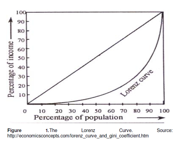
(In order to draw the curve from which the Gini Coefficient may be estimated, the percentage of income given to income recipients is measured on the vertical axis. The income recipients are arranged in percentiles on the horizontal axis. Income recipients are ranked from the poorest to the richest mainly from the left to the right. Thus a certain percentage of the population of the poorest group receives a certain percentage of the income. The line of complete equality is represented by the 45° line which is also called the egalitarian. This complete equality will only occur if “A” percentage of the population received “A” percentage of the income. The curve of the perfect inequality represents the case where one person has 100% of the income (represented by the curve angle DCB). The space between the Lorenz curve and the 45° line represent the area of concentration, that is, enclosed by the theoretical egalitarian and the observed Lorenz curve.
The Gini coefficient is the ratio of this area to the total area under the line of equality. The simplest method of computing this is by taking the sum of the area under all the trapezoids such as WXYZ and subtracting it from the area under L. As a measure of income concentration, the Gini Coefficient ranges from 0-1. The larger the coefficient the greater the inequality; the figure 0 (zero) represents perfect equality, 1 represents perfect inequality. Alternatively, Gini Coefficient may be measured by the area of concentration divided by the area of triangle DCB. The shape of the Lorenz curve will indicate the degree of inequality in the income distribution. The curve definition must touch the 45° line at the lower left corner and upper right corner (as can be observed in the Hypothetical Lorenz Curve).
Problems
The Lorenz Curve can intersect so that different curves can give the same Gini Ratio because of difference in inequality of the range. The extreme nature of the reference standard perfect equality makes the measure insensitive to changes in income distribution. The insensitivity is greatest for changes in the incomes of low income groups which may be small in absolute terms but still important in percentage terms to the poor households themselves and redistribution in policy terms. To avoid the arbitrariness this may present in Lorenz Curve, different particular parts of the curved are looked at. The poorest 20 or 40% may be checked to know how the poor are faring or top 5, 10, 20% to check the concentration of wealth.
Bio-graphic and socioeconomic characteristics of respondents
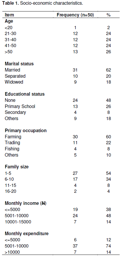
Of the 50 women interviewed, only 2% were teenagers, 26% of them were above 50 years in age while 72% ranged between 21 to 50 years. This indicates early marriage and long child producing /caring periods. This indirectly means that the women are active for a long period in their lives, often keeping the home and working on the farm.
The long procreation period shows that there would be break periods in the productivity of the women; such many time outs would reduce her overall productive capacity apart from weakening their health (Santhya et al., 2010). The average age of women is 41 years while the range is 30 years; that the women start out early in life to fend for their families indicate that they would have gained a lot of practical experience which if tapped could lead to an increase in income and as such raise their living standards.
Most of the women (62%) were married; 20% of them were separated from their husbands while 18% of them were widows. None of them was single and some of the married women lived separately from their husbands (who pay occasional visits) so they still have to cater for the family. A proportion of 38% of the women were heads of their homes which implies that all the financial, physical, social, psychological burdens would be borne by them. The heaviest of all is the economic burden which hangs on their necks.
These women are usually the poorest of the poor; since their capacities will be over stretched. The proportion could be higher because some married women do live separately with kids. About 50% of the married women leave separated from their spouses. The reasons they gave for this include the presence of another wife elsewhere and husband’s occupation involving travelling. Consequently the burden of survival falls on them. This shows that while more men are leaving farming for the women; their burden becomes heavier. This scenario explains why poverty is feminized in this region.
Less than 50% of the women had no formal education, which indicates a high level of illiteracy among the women. Some 26 percent have primary level education, 8 percent got to the secondary school level while another 18 percent attended teacher training college or modern school. The low level of education among the respondents would affect their innovativeness, rate of adoption and response to change. All these being low would affect their productive capacity and help them no further than what they are now. The prevalent low level of education has not deterred them from being involved in different activities as a source of livelihood for them and their families. The women consider farming (30%), trading (26%), fishing (12%) and those who are civil servants such as teachers (14%) as primary sources of income. However all of them have farms, the product of which they sell and consume. They also make crafts such as mats. None of them saw house-keeping as a productive job nor do they use it as a deterrent to their occupations. The fact women do not consider housekeeping to be a productive activity is the reason why women’s economic contributions at the national level are under-reported. Tshuma and Jari (2013) found that the informal sector is a source of income for households in poor communities. The average income by month is N6,680. About 54% of the women earn less than this while the remaining 46% earn more. The average monthly expenditure is N6,772.34. This figure is higher than the monthly income, which suggests that the level of indebtedness would be high. The expenditure amount represent about 90% of the income which implies no savings and the households are probably borrowing to survive (Table 1).
Time use of women in rural riverine areas
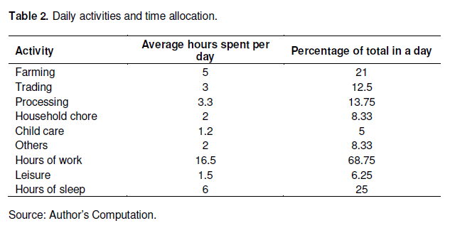
This is considered in two ways: the average number of hours which women spend on specific activities and a comparison of what men and women do at particular periods of the day. In the latter, questions were asked on activities of both husband and wives at particular periods, while the former involves calculating average hours allocated to each activity for all women. Most of their time is spent working: 6.25% on leisure, 25% on sleeping and68.75 on working (Table 2). Further analysis shows that men have more hours of sleep, leisure and shorter hours of work (Appendix 1). According to Blackden and Wodon (2006), overlooking the differences in men’s and women’s contributions to “household time overhead” can lead to inappropriate policies which have the unintended effect of raising women’s labor burdens while some-times lowering those of men.
Determination of respondents in poverty
This begins with drawing the poverty line. Ideally this line should be defined in terms of household per capital income but the basic needs approach specifies that the mean household expenditure per month be used. Thus households below the poverty line will be termed poor while those above will be termed none poor.
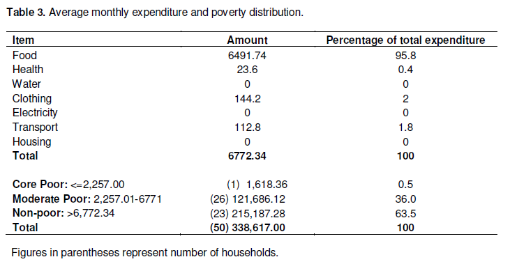
For this particular study, poverty line was established based on the mean household expenditure per month on some basic needs: food, health (medication), water, clothing, electricity, transport, and housing. Poverty is then calculated identifying core poverty group, moderate poverty as well as the non-poor groups. A core poverty household is identified if it spends less than one-third of the average expenditure on basic needs while a moderate poverty household spends less than two thirds of the average expenditure on basic needs. In addition, the non-poor is identified if it spends more than the average expenditure by households.
The average expenditure on basic needs of households was calculated by taking the average expenditure of all the respondents on the basic requirement (mentioned above) which includes food and non-food items. Table 3 shows the average amount spent by each sampled house in the study area where food is shown to constitute the bulk of monthly expenditure of the households. The poverty line stands at N6772.34. Following the assumption above the core poverty line is N2,257.00 while the moderate poverty line is N4,514.89. From the monthly expenditure of each household in the study, it is shown that only a household falls in the core poverty group. It can be seen that only two percent of the sample is in core poverty while 22% are moderately poor. In all a total of 54% could be said to live in poverty while 46% are not poor. Ologbon et al. (2014) found that 60% of households in the riverine areas of southwestern Nigeria lived in poverty. The percentage of the total expenditure spent by those above the poverty line is 63.5% while the remaining 36.5% is spent by those below it.
Poverty depth measurement
To show the poverty profile of the respondents more clearly, other poverty indicators were used. They include:
Head count index: This is the proportion of the population whose measure of standard of living, (consumption) is less than the poverty line. It is useful as quick indication of the scope of the poverty problem, though it is insensitive to differences between individuals in the depths of severity of their poverty. Head count index is poor (people below the poverty line) as a percentage of total sample size. It is given by:
(Poor × 100) / Total sample = (27 × 100) / 50 = 54%
Poverty gap index: This is the difference between the poverty line and the mean expenditure of the poor expressed as a ratio of the poverty line. It is also called the Income Gap Ratio. It gives a good indication of the depth of poverty but does not capture its severity. It is given by:
(Poverty line - Mean expenditure of the poor) / Poverty line
= (N6772.34 – N4566.83) / N6772.34
= N2,205.51 / N6,772.34
= 0.325
≈ 0.33
The implication of this is that the poor expend a third of
what the non-poor spend in a year or the non-poor earn three times more than the poor although the figures may give the impression that there is not much gap between the chosen poverty line and the average monthly expenditure of the household.
Determination of the Lorenz
The Gini coefficient which shows the severity of the poverty curve was calculated using the formula below
Gini Coefficient: =1-(Xi+1 – Xi)(Yi + Yi+1)
Where:
Xi = Percentage of household
Yi = Cumulative percentage of expenditure distribution
This was calculated to be 0.22 which implies that there is an even spread in the expenditure around the 45 line to some extent. Particular points on the Lorenz Curve were checked to see how the different groups of people are faring. For this study, the lowest 10 and 20% of the sample were also checked; and the top 10 and 20% of the sample are also checked. The first 10% cover a total of 3.81% of the total expenditure, while the first 20% spends a total of 10.1% of the total expenditure. The top 10 and 20% spend 18.59 and 32.88% of the expenditure respectively.
Productivity analysis
Correlation analysis of production function
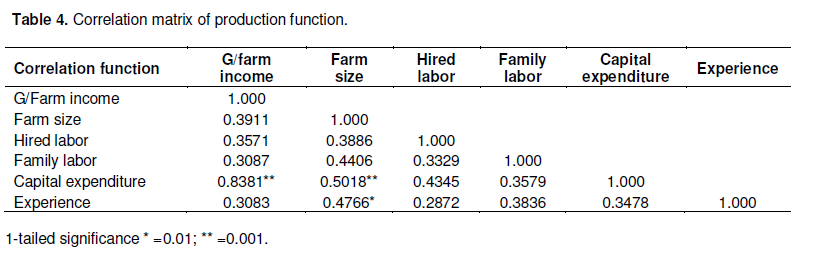
The correlation matrix below (Table 4) shows that the variables are all positively correlated. Capital expenditure is shown to be highly correlated with land or farm size and income. This shows that an increase in capital expenditure per hectare will increase the income of the farm family. Experience is also highly correlated with land size, implying that being an experienced farmer will help to increase output per hectare of land. Others though positive are weakly correlated to income.
Resource productivity analysis
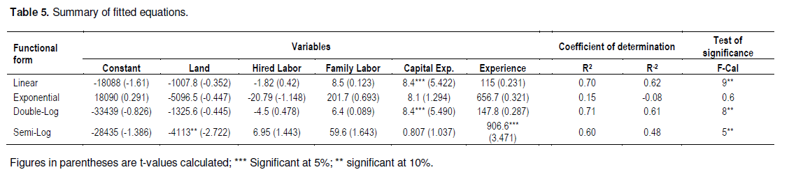
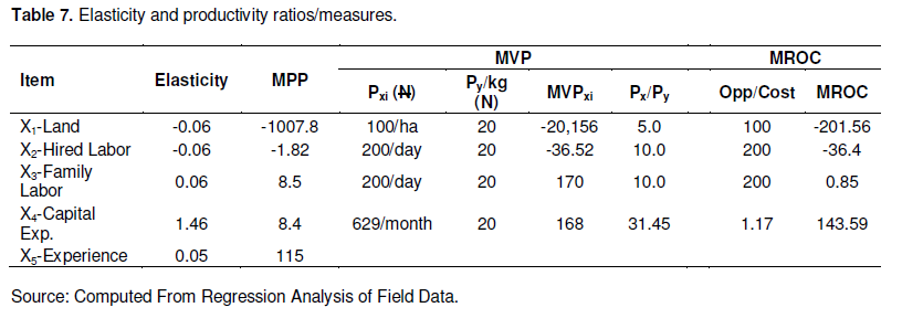
Four functional forms (Linear, Exponential, Double-Log and Semi-Log) were fitted in the regression variables to estimate their effects on farm income; based on the criteria stated earlier, the linear function was found to be the best hence it was chosen as the ‘lead equation’. The aim of this section therefore is to find the marginal physical product, elasticity of production, opportunity cost, marginal returns to opportunity cost ratio, and marginal value product based on the equation. With these it is possible to investigate if resources are being used optimally and find out the nature of returns to scale. The expressions of the equations in explicit forms are presented in the Table 5.
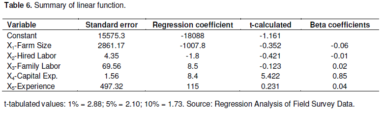
The coefficient of determination of the lead equation is 0.70 which means that 70% of the total variation in income is explained by the independent variables while the remaining 30% could be explained by such variables as weather, technology which are not included in the equation. The f-ratio shows the overall significance of the equation and it is significant at both 1 and 5%. This shows that the coefficient of determination obtained for the equation is significantly different from zero.
The coefficient of land size and hired labor are both negative and insignificant at the critical level of test chosen. This implies that increasing the farm size could have a negative effect on income since such could lead either to underutilization of land, over use of land due to intensive mono-cropping system or inefficiency; or land is not very productive and diminishing returns has set in. Labor increase might also affect income negatively. These results are contrary to the a priori expectation. Capital expenditure (X4) is the only significant variable at the critical levels tested. It is also positive which implies that the variable cost of farming is low and an increase in it would lead to increase in farm output and ultimately farm income; the implication also is that farming is capital intensive. Family labor and experience are positive but not significant. An increase in both of them should raise output per hectare but the results run contrary to a priori expectation suggesting that allocation of family own resources may be in line with other objectives rather than farm income. The Beta-coefficients is used to differentiate the net effect or relative importance of each independent variable to the dependent variable. It shows the increase or decrease in the dependent variable (standard deviation units) resulting from an increase of a standard deviation unit in each independent variable. For the study it reveals that the highest influence of change in income or output is given by capital. Family labor and experience contribute very marginally positively while the net effect of farm size and hired labor is negative (Table 6). This indicates diminishing marginal returns with respect to labor resources.
Elasticity of production, marginal physical product, marginal value product and marginal returns to opportunity cost
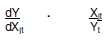
The elasticity of production shows the change in output relative to a unit change in input; other inputs remaining constant. A ratio greater than unity implies that change in output out paces change in input; and production is said to be relatively elastic. A ratio equal to unity implies that output changes at the same rate as input, and production elasticity is said to be unitary. While a ratio less than unity indicates that the proportionate change in output is less than that of input and production is said to be inelastic. The elasticity of a linear function is given by:
The elasticity of the dependent variable is not necessarily constant. The elasticity of production in this case is given by:
Ei = biXÌ…i / YÌ…
Where XÌ… and YÌ… are the means of input and output respectively.
The elasticity of land was found to be -0.006, the same goes for hired labor. Both being negative and less than one indicate inelasticity of production with respect to them. Family labor and experience have elasticity of 0.06 and 0.05 respectively again indicating inelastic production though positive. The elasticity of production with respect capital expenditure is 1.46, it is positive and above 1 showing that production is elastic. The sum of elasticity gives 1.44 indicating increasing returns to scale.
Marginal Physical Product (MPP) shows the marginal change in output with respect to a marginal change in input. The partial derivative of the function with respect to each input gives MPP. It gives the maximum level of input used in getting maximum output. For the linear function, the MPP is the same as the regression coefficients. The variable X3, experience, gives the maximum MPP value. Though family labor and experience (X3 and X5 respectively) show the highest MPP levels, their elasticity are small because they are not easily increased.
Production is said to be efficiently organized under conditions of competition in the input and output markets when the marginal value product is equal to the marginal factor cost for each of the inputs used. That is, for a given level of technology, prices of both input and output, the marginal value productivity is an instrument for judging the efficiency of resource use when related to prices of inputs. The marginal value product of hired labor and land are higher than the input prices which shows that they are over utilized. They are negative so need to be reduced to increase output or shift from current plots being used. Family labor and capital expenditure are being under-utilized; they need to be increased to give higher output hence income. An input is efficiently utilized if its marginal value product is just sufficient to offset its marginal factor (input) cost. The marginal value product and the input price or marginal factor cost is a basic condition that must be satisfied to obtain efficient resource use. The marginal value productivities of resources therefore provide a framework of policy decision on resource adjustment. A positive marginal value productivity shows that output can be increased by using more of that resource while a negative value shows the opposite. The Marginal Value Product (MVP) is the product of the MPP and the price of the output.
(MPP)Py = Pxi
Pxi = Price of inputs X1, X2, X3, X4, X5
Py = Price of output, Y
The marginal factor cost is the cost of acquiring an additional unit of that input. The average prices paid for inputs were used as proxies for marginal factor cost.
Marginal Returns to Opportunity Cost (MROC) ratio measures efficiency in resource use. A ratio greater than 1 indicates that little of the particular resource is being used under the prevailing price situation. Optimum utilization of resources occurs when the marginal return to opportunity cost ratio is equal to unity. The opportunity costs of the various resources are approximated by their market prices. For land the annual rental value for agricultural use in the study area is taken as an estimate of its opportunity cost; the same applied to family labor. Capital expenditure that is valued in Naira terms, the opportunity cost of N1.00 of capital is taken as N1.00 plus the current annual interest rate (17%) (Table 7).
This study has attempted to examine the source of rural women’s poverty, the severity and the efficiency of resource use in their farming activities. It is generally agreed that women are more into food crop farming and that majority of the food eaten in Africa and Nigeria in particular is a result of the activities of these women, yet returns to resources is low. It is recommended that government and other development agents need to identify different rural communities, particularly those which seem to be locked-in like the study area; study them and develop particular programs or projects in response to their particular problems. Poverty and productivity need to be attacked simultaneously because they are intertwined and affect each other. Such projects should involve the beneficiaries at every stage while its implementation should be closely monitored and evaluated on a regular basis. If measures are taken as recommended, the efficiency of the women will be increased; income will improve and poverty reduced.
The authors have not declared any conflict of interests.
REFERENCES
|
Adekanye TO (1983). Women in Food and Agriculture in Nigeria: Some considerations For Development. Banglad. J. Agric. Econ. 6(1):61-68.
|
|
|
|
Adekanye TO (1984). Women in Agriculture in Nigeria: Problems and Policies for Development. Women Stud. Int. Forum 7(6):55-63.
|
|
|
|
Bhat TA, Lone SA (2013). Soviet Healthcare System in Kazakhstan. J. Eurasian Stud. 5(1):56-116.
|
|
|
|
Blackden M, Wodon Q (2006). Gender, Time Use, and Poverty in Sub-Saharan Africa World Bank Working Paper 73 Washington D.C.
|
|
|
|
Braun J, Gatzweiler FW (2014). Marginality—An Overview and Implications for Policy in Braun VJ and Gatzweiler FW (Eds.). Marginality: Addressing the Nexus of Poverty, Exclusion and Ecology Springer Dordrecht Heidelberg.
Crossref
|
|
|
|
Durmont R (1969). False Start in Africa 2nd Edition Fredric A Preger, Publishers New York, Washington.
|
|
|
|
Mcnamara RS (1975). The Assault on World Poverty The John Hopkins University Press.
|
|
|
|
Ogbonna KI, Okoroafor DE (2004). Enhancing The Capacity Of Women For Increased Participation In Nigeria Main-Streaming Agriculture: A Re-Designing of Strategies Paper prepared for presentation at the Farm Management Association of Nigeria Conference, Abuja, Nigeria. Oct. 19-21.
|
|
|
|
Ogunlade Y (2010). Impact of Water Hyacinth on Socio-Economic Activities: Ondo State As A Case Study In: Proceedings of the International Conference on Water Hyacinth, 27 Nov - 1 Dec 2000, New Bussa, Nigeria . pp. 175-183.
|
|
|
|
Ologbon OAC, Idowu AO, Oyebanjo O, Akerele EO (2014). Multidimensional Poverty Characteristics among Riverine Households in Southwestern Nigeria. J. Sustain. Dev. Afr. 16(6).
|
|
|
|
Olorunlana FA (2013). State of the Environment in the Niger Delta Area of Ondo State Paper presented at the 1st Interdisciplinary Conference, AIIC, 24 – 26 April, Azores, Portugal.
|
|
|
|
Olubanjo, OO, Akinleye SO, Adekoya MI (2005). Socio-Economics of Fisher-Folks in the Capture Fisheries of the Ogun Waterside Area, Nigeria.
View
|
|
|
|
Santhya KG, Ram U, Acharya R, Jejeebhoy SJ, Ram F, Singh A (2010). Associations between Early Marriage and Young Women's Marital and Reproductive Health Outcomes: Evidence from India. Int. Perspect. Sex. Reprod. Health 36(3):132-139.
Crossref
|
|
|
|
Tshuma MC, Jari B (2013). The informal sector as a source of Household Income: The case of Alice town in the Eastern Cape Province of South Africa. J. Afr. Stud. Dev. 5(8):250-260.
|
|
|
|
Vijayakumar S, Olga B (2012). Poverty Incidence and its Determinants in the Estate Sector of Sri Lanka. J. Competitiveness 4(1):44-55.
Crossref
|
|
|
|
World Bank (1996). Nigeria: Poverty in the Midst of Plenty- The Challenge of Growth with Inclusion. World Bank Poverty Assessment: Population and Human Resources Division, Western Africa Department Africa.
|
APPENDIX
.png)
.png)