ABSTRACT
This study empirically examined the effect of research and development on agricultural sector growth in East African Community from the year 2000-2014. According to the endogenous growth theory, research and development leads to increase in the stock of knowledge which in turn has got spill over effects hence leads to economic growth. However, little is known on the effect of R&D on the agricultural sector in the EAC hence the study sought to bridge this knowledge gap. The objective of this study was to determine the effect of agricultural research and development on agricultural sector growth. Panel data analysis was used with stationarity test conducted using Levin-Lin- Chu panel unit root test. Stationarity test showed that some variables were stationary at level while others were stationary after first differencing. Random effects regression results showed that explanatory variables had a positive and significant relationship with the dependent variable and the recommendations are: That R&D to be allocated more funds; more research scientists and agricultural labourers to be employed, trained and motivated through better remuneration and good work environment; R&D based knowledge to be disseminated to the public through publications; firms to train agricultural labourers on how new technologies are being used and also to allocate them duties and responsibilities that match their skills and that agricultural capital costs be subsidised.
Key words: Agricultural sector growth, research and development, East Africa Community, economic growth, stationarity, and regression results.
Research and development (R&D) is a systematic and creative work undertaken in order to increase the stock of knowledge, including knowledge of man, culture and society, and the use of this knowledge to devise new applications. Research and development activities include basic research, applied research and experimental development (Cororaton, 1999; Bronzini and Paolo, 2006). Research and development represents a large and rapidly growing effort in both industrialized and semi-industrialized nations. In 1997, the USA spent $151 billion on industrial R&D and $32 billion on military R&D. Similar ratios exist for economically advanced countries, such as Germany, France, the United Kingdom and Japan (Svensson, 2008). In order to compete in the international marketplace, rapidly industrialising countries such as Korea, Indonesia and Brazil have national policies in place for developing indigenous R&D (Svensson, 2008). Major countries not politically aligned with the western powers, notably Russia, China, and India, and to a certain extent, France and Israel have significant levels of R&D for defence purposes, in order to be technologically and logistically independent from western sources and to export arms to third world countries (Bronzini and Paolo, 2006; Svensson, 2008).
South Africa, Iraq, and North Korea spent inordinate amounts of their limited GNPs for military purposes in the 1990s (Svensson, 2008). The reason for this increased emphasis on R&D is that it creates new or improved technology that in turn can be converted into a competitive advantage at the business, corporate, and national level (Svensson, 2008). While the process of technological innovation is complex and risky, the reward can be very high. If technology can be safeguarded as proprietary and protected by patents, trade secrets, non-disclosure agreements, etc., the technology becomes the exclusive property of the company and the value is much higher (Svensson, 2008). In earlier neo-classical theory, knowledge was regarded as an exogenous variable that, together with a company’s input, goods, labour and capital, affects productivity (Solow, 1956; Swan, 1956). In endogenous growth theory, on the other hand, investments in R&D that provide new knowledge are seen as an important factor that explains growth and increased productivity (Romer, 1990). This theory regards new technology not only as an exogenously produced input good that the company utilises, but new technology can also be created within the company.
In endogenous growth theory, investments in R&D can provide long term growth and lead to rising returns to scale (Romer, 1990; Jones, 2004). This is because previous R&D investments that were made to generate a specific knowledge do not need to be made again. Research and development investments are irreversible investments and subject to an uncertainty (Jones, 2004; Sadraoui et al., 2014). R&D that is performed by a company often leads to new and/or improved goods and services that the company then sells (Bronzini and Paolo, 2006; Svensson; Kim, 2011, 2008). The company may not be able to utilise some of the results of its R&D and these may then be transferred through various channels (imitation, personnel who change jobs, licensing, cooperation between companies) to other companies (Idea and Svensson, 2008). Mansfield (1981) estimated that the cost of imitating a product is 65% of the original innovation costs. Performing R&D also leads to further training for the company’s personnel. In addition, the company becomes better at absorbing knowledge that is generated at universities and other companies (Cohen and Levinthal, 1989; Geroski, 1995).
This improves the ability of a company to utilise spillovers from other companies. Many observers, including Callon (1994) pointed out that knowledge generated as a result of R&D is not a public good that can be utilised by everyone as a certain form of education and training and the right networks are required to be able to understand and utilise new knowledge generated by others, thus associated with a cost. Another characteristic of knowledge is that it cannot always be codified but is “tacit”, that is, the researchers/scientists know more than they can put into words (Rosenberg, 1990; Pavit, 1991). In general, this requires the participation of the researchers concerned if new research results are to be converted into innovations. The East African Community (EAC) is an intergovernmental organisation comprising five countries in the African Great Lakes region in Eastern Africa: Burundi, Kenya, Rwanda, Tanzania, and Uganda. The organisation was originally founded in 1967, collapsed in 1977, and was officially revived on 7th July 2000 (Gisore et al., 2014). All five of the East African community countries have shown their commitment through the formulation of relevant and the establishment of bodies in charge of higher education, science, technology, and innovation (Tumushabe and Mugabe, 2012).
There are bodies dedicated to higher education research, science and technology already in place in East Africa; the National Council for Science and Technology (NCST) in Kenya, the Commission for Science and Technology (COSTECH) in Tanzania, the National Council for Science and Technology (UNCST) in Uganda, the Ministry of Education in Rwanda, and the Ministry of Higher Education and Scientific Research in Burundi (Tumushabe and Mugabe, 2012). In addition, the EAC states allocate funds for R&D for example during the period of 2000 to 2014, Burundi spent an average of 0.2% of its GDP on R&D, Kenya spent an average of 0.67% of its gross domestic product (GDP) on R&D, Uganda spent an average of 0.43% of its GDP on R&D, Tanzania spent an average of 0.36% of its GDP on R&D while Rwanda spent an average of 0.22% 0f its GDP on R&D (Author computations). These point to recognition of the role of higher education research, science and technology transfer in economic development in the EACS.
EAC states have formulated policies to guide research and innovations and technology transfer, for example in Kenya, there is facilitation of acquisition of intellectual property rights by scientists, researchers and innovators; in Tanzania, there is the high level scientific research and technological trainings, motivation and retention programmes which include provision of attractive terms and conditions of service for scientists and technologists, while in Rwanda, there is regular audit of research and knowledge transfer capacity to enable the quality and extent of research and knowledge transfer activity be properly assessed, and in Uganda, there is support for local innovation and scientific excellence by funding national research priorities and providing infrastructure for technology generation and incubation and these if fully implemented, would see great accomplishments in higher-education research, science and technology activities, as well as increased collaborations with industry that would lead to the economic development of these nations (Gisore et al., 2014; Tumushabe and Mugabe, 2012).
This study is of importance to policy makers to come up with research and development policies that are relevant to the agricultural sector in the EAC. The study covered East African Community states and the period of study was from the years 2000 to 2014. Due to the data gaps for some years before the year 2000 in Uganda, Rwanda and Burundi which could be attributed to political instabilities that these countries faced in the 1970s and 1990s, the study was limited to the period of 2000 to 2014 since data for this period was available for the study. The motivation for this study is to bridge the knowledge gap that exists on the relationship between research and development and the agricultural sector in the East African Community despite the commitments that have been shown towards research and development.
Theory
Sheshinski (1967) theory emphasise the spill-over effects of increased knowledge through learning by doing as the source of knowledge. The theory says that the source of knowledge or learning by doing is each firm’s investment and an increase in a firm’s investment leads to a parallel increase in its level of knowledge. The theory also says that the knowledge of a firm is a public good which other firms can have at zero cost. Thus, knowledge has a non-rival character which spills-over across all the firms in the economy. This stems from the fact that each firm operates under constant returns to scale and the economy as a whole is operating under increasing returns to scale. Romer (1986) showed later that an equilibrium rate of technological advance can be determined in this case if the competitive framework can be retained. But such a growth rate would typically not be Pareto optimal. In general, the competitive framework may not be valid if new ideas depend particularly on purposive R&D and if innovations spread only progressively to other producers.
King and Robson (1989) theory emphasise learning by watching. The theory says that investment by a firm represent innovation to solve the problems it faces. If it is successful, the other firms will adapt the innovation to their own needs. Thus, the externalities resulting from learning by watching are a key to economic growth. The theory says that innovation in one sector of the economy has the contagion or demonstration effect on the productivity of other sectors, thereby leading to economic growth. The theory concludes that multiple steady state growth paths exist even for economies having similar initial endowments and that policies that increase investment should be pursued. This was supported by Scott (1989) who said that on-going production processes are seen as heritage from the past. Increase in production can be brought about by changing production processes and by changing existing economic arrangements, which requires investment outlays to be made.
At the same time, every transformation implies problem solving from which people learn. However, learning by watching is not automatic as the theory almost inevitably suggests. In fact it depends on the organisation of industry and trade and the way firms take advantage of these opportunities. This was according to Porter (1990) who said that competitive advantage emerges from close working relationships between world class suppliers and the industry. Firms gain quick access to information, to new ideas and insights, and to supplier innovations. They have the opportunity to influence suppliers’ technical efforts as well as serve as test sites for development work. The exchange of R&D results and joint problem solving leads to a faster and more efficient solution. Suppliers also tend to be conduits for transmitting information and innovations from firm to firm. Through this process, the pace of innovation within the entire national industry is accelerated. Romer (1990) model identifies a research sector specialising in the production of ideas and this involves human capital along with the existing stock of knowledge to produce ideas or new knowledge.
The new knowledge enters into the production process in three ways. First, a new design is used in the intermediate goods sector for the production of a new intermediate input. Second, in the final sector, labour, human capital and available producer durables produce the final product. Third, a new design increases the total stock of knowledge which increases the productivity of human capital employed in the research sector. However, the increase in the stock of knowledge due to a new design may be limited through patenting and lack of proper dissemination of knowledge. While Romer’s approach postulates innovation of new capital goods that make production of final goods less costly, Grossman and Helpman (1991) together with Aghion and Howitt (1992) developed models where innovation improves the quality of existing varieties of capital goods. However, the shortcoming in Romer’s (1990) model is that there is an infinite life for a R&D patent. This contradicts facts in real life, which are usually less than twenty years.
Empirical literature review
Bozkurt (2015) analysed the relationship between research and development expenditure and economic growth in Turkey using vector autoregressive model and Granger causality test. He found that there was evidence of Granger causality from gross domestic product to research and development while there was no evidence of Granger causality from research and development to gross domestic product. He went further and said that as economic activities and economic growth rate increases, research and development also increases for sustainability. He therefore concluded that information economy and sectors with high technology are very important for economic development and that it is also obvious that achieving development and growth is not easy without research and development. According to Sadraoui et al. (2014) who analysed the causality between R&D collaboration and economic growth by using the data of 32 industrialized and developed countries for the period of 1970 to 2012 got results that support the argument that there is a strong causality between economic growth and research and development collaboration.
On the contrary, non-causality between research and development collaboration and economic growth could not be ignored in several contexts. The results showed such a relationship that Granger causality test with one or two variants could not be defined easily. In addition, Inekwe (2014) in his study that covered developing countries in which 66 countries were covered during the period of 2000 to 2009 and the countries were divided into economies with higher level of income and with mid and lower income levels, found that R&D expenditure had a significant effect on economic growth in developing countries and that there was a positive effect of research and development on economic growth in countries with higher and medium income levels but insignificant relationship between research and development expenditure and economic growth was found in the countries with lower and medium income levels. In addition, Fuglie and Marder (2015) in their study on the effect of the adoption of improved crop varieties of 20 crops from 1970 to 2010 which covered 37 sub-Saharan countries found that the improved varieties had a major positive impact on agricultural productivity.
Rada and Schimelpfenig (2015) conducted a study on the determinants of total factor productivity growth in India and they found that public research made major contributions to the total factor of productivity growth. According to Kadir et al. (2015) who investigated the relationship between research and development expenditures and economic growth in Turkey using data covering the period of 1990 to 2013, found that there was no long-term relationship between real research and development expenditure and economic growth series based on the tests that were conducted. In addition, he also found that there was no causality relationship between research and development expenditure and economic growth in consequence of Granger causality test that was conducted.
According to Rao et al. (2016) in their meta-analysis of 2829 specific estimates of returns to agricultural research and development programs and projects in 78 countries found that returns to research had not declined over time and that developing countries generally had higher rates of return (median of 41%) than developed countries (median return of 34%). In addition, Pardy et al. (2016) in their analysis on the estimates of returns to agricultural research and development in 25 countries in Africa from 1975 to 2014 found high rates to agricultural research and development with a median of 35% and a mean of 42%. In summary, empirical studies on the effect of R&D on growth have led to different results in different economies; hence, they have been inconclusive. In addition, studies on embodiment of technology in capital and labour are also lacking hence studies needs to be done to close these gaps.
Theoretical framework
This study was based on Romer (1990) model of technological change. The model identifies a research sector specialising in the production of ideas. This sector involves human capital along with the existing stock of knowledge to produce ideas or new knowledge. To Romer, ideas are more important than natural resources. He cites the example of Japan which has very few natural resources but it was open to new western ideas and technology. Therefore, ideas are essential for the growth of an economy. These ideas relate to improved designs for the production of producer durable goods for final production. In the Romer model, new knowledge enters into the production process in three ways. First, a new design is used in the intermediate goods sector for the production of a new intermediate input. Second, in the final sector, labour, human capital and available producer durables produce the final product. Third and a new design increase the total stock of knowledge which increases the productivity of human capital employed in the research sector.
While Romer’s approach postulates innovation of new capital goods that make production of final goods less costly, Grossman and Helpman (1991) together with Aghion and Howitt (1992) developed models where innovation improves the quality of existing varieties of capital goods. Romer (1990) model is based on the following assumptions: first, economic growth comes from technological change, secondly, technological change is endogenous, thirdly, market incentives play an important role in making technological changes available to the economy, fourthly, invention of a new design requires a specified amount of human capital, fifthly, the aggregate supply of human capital is fixed, sixthly, knowledge or a new design is assumed to be partially excludable and retainable by the firm which invented the new design. Seventhly, technology is a non-rival input, that is, its use by one firm does not prevent its use by another.
Eighthly, the new design can be used by firms and in different periods without additional costs and without reducing the value of the input. Ninth, it is also assumed that the low cost of using an existing design reduces the cost of creating new designs and lastly, it is assumed that when firms make investments on research and development and invent a new design, there are externalities that are internalised by private agreements. However, the shortcoming in Romer’s (1990) model is that there is an infinite life for a R&D patent; this contradicts facts in real life, which are usually less than twenty years.
In the neo-classical model, the stock of ideas, A is assumed to change over time, separately from the production decision. For example, in the Cobb-Douglas production function, we write:
Y= AKaL1-a (1)
The Romer (1990) model describes how capital stock, K and labour, LY combine using a stock of knowledge, A, if A is assumed to represent a stock of knowledge.
Y=Ka (ALY) 1-a (2)
where a is a parameter between 0 and 1. For given level of technology, A, the production function shows constant returns to scale in K and LY, but if A increases, then there will be increasing returns. If capital, labour, and the stock of technology all double, then output more than doubles.
The Romer (1990) model could be developed assuming that the savings rate is given exogenously.
Capital accumulation is:
= skY-dK (3)
Labour grows exponentially at a constant rate, n:
=n (4)
In the neoclassical model, the productivity term A grows exogenously at a constant rate. In the Romer (1990) model, growth in A is endogenous. At is the stock of knowledge at time, t. It changes as a function of the number of innovators.
= LA (5)
So labour can be used either for innovation or production. The rate of innovation might be constant or it might be positive function of the past stock of knowledge, or, if there are diminishing returns to the application of science, it might be a decreasing function of the stock, Romer (1990) asserts that,
=δAΦ (6)
where Φ>0 means that the productivity of research increases with the stock of A and Φ<0 means that productivity is declining. Noticing that R&D tended to concentrate in a few central locations, Romer (1990) added a term, Lλ, to his model of the stock of knowledge. If λ<1, then researchers were wasting their time re-discovering knowledge that was already known. If λ>1, then there were complementarities (positive knowledge spillovers) in research. If Φ>0, then current scientists benefit from the knowledge of earlier science. In the Romer (1990) model, if a constant fraction of the population is employed in R&D, the model follows the neoclassical model in predicting that all per capita growth is due to technological progress.
GY=gk = gA (7)
Per capita output, the capital-labour ratio, and the stock of knowledge all grow at the same rate. If there is no technological progress, then there is no growth.
gA= /A=δ /A1-Φ (8)
The growth rate of A is constant only if the numerator and denominator of this expression are growing at the same rate. Taking logs and derivatives of both sides, this requires that:
0=λ A/LA-(1-Φ) /A (9)
Along a balanced growth path, the growth rate in the number of researchers equals the growth of population (otherwise it eventually exceeds the population.) That is, A/LA=n. Substituting this into 1.8 yields:
gA=λn/1-Φ (10)
This says that long run growth depends on the growth rate of innovators and the innovation production function. This means that if λ=1 and Φ=0 so that the productivity of researchers is constant at δ, then the productivity of a researcher today is independent of the stock of ideas that have been discovered in the past. The production function for knowledge is:
=δLA (11)
Notice, if the output of new knowledge is constant, at 100 new ideas per period, and unrelated to the stock of knowledge is getting larger, then the growth rate of the stock of ideas falls over time, approaching zero. In order to generate growth, the number of new ideas must be expanding over time for example the number of researchers is increasing. In the neoclassical model, a higher population growth rate reduces the level of per capita income along a balanced growth path. More people means that more capital is needed to keep K/L constant, but capital runs into diminishing returns. In the Romer (1990) model, people create new innovations which are non-rivalrous, so everyone benefits. In the original model, assumed that λ=1 and Φ=1, so that:
=δLAA (12)
and
/A=δLA (13)
In this case, the productivity of research is proportional to the existing stock of ideas:
=δA
In this form, the productivity of researchers grows over time even if the number of researchers is constant. In case of a permanent increase in the R&D share (assuming that λ =1 and Φ=0), temporarily, technological progress, =δLA exceeds population growth, n, so the ratio, LA/A declines over time. As this ratio declines, the rate of technological progress gradually falls until the economy returns to a balanced growth path, where gA=n. The level of technology is permanently higher as a result of the permanent increase in R&D. There is a scale effect in levels; a larger world economy is a richer economy.
Panel model estimation
The basic regression equation that was used to investigate the relationship between R&D and agricultural sector growth was of the type:
lnYi,t =β1lnREAi,t + β2lnREOi,t +µi +vt +εi,t
where Yi,t is the dependent variable that is agricultural sector growth (Agricultural output). REAi,t is the agricultural R&D. REOit is the R&D in other sectors apart from the agricultural sector. µi represents unobserved country specific effects. vt represents unobserved time specific effects. εi,t is the error term.
Data
The data that was used in the study was a panel data that consisted of a panel of five countries covering the period of 2000 to 2014. The dependent variable was agricultural sector growth (agricultural output) while the explanatory variables were agricultural research and development, research and development in other sectors (apart from the agricultural sector). Agricultural output was used as the proxy or measure of the agricultural sector growth while agricultural research and development expenditure was used as a measure of agricultural research and development. The sources of data were purely secondary sources. Data on agricultural sector growth (agricultural output) was gotten from the websites of the member countries National Bureaus of Statistics and their Statistical Abstracts in addition to the World Development Indicators website. Data on agricultural research and development (Agricultural research and development expenditure) was gotten from Agricultural Science & Technology Indicators (ASTI) website and from the member countries National Bureaus of Statistics websites. Data on research and development in other sectors (Research and Development expenditure in other sectors) was computed by getting the difference between total research and development expenditure and agricultural research and development expenditure. Data on total research and development expenditure was readily available on World Development Indicators website and World Data Atlas website.
Analysis
Various tests were first conducted to ensure that the results were unbiased and are the ones that could be relied on. Unit root test was done to establish stationarity of a data series. Panel unit root test was conducted to avoid analysing non stationary data at level which in turn could lead to spurious results or results that do not make sense. Data found to be non-stationary at level were different for stationarity to be achieved. Stationary data were then analysed because the results were now sensible. Levin et al. (2002) developed a unit root test for panel data. Co-integration refers to the long-run linear movement of two variables that are stationary after differencing. When the linear combination of the two variables is I(0), then the variables are said to be co-integrated. Differencing data to achieve stationarity leads to lose of long run relationship between variables and so co-integration test is being conducted to check whether the variables have got long run relationship or not. Pedroni (1999) developed a residual-based panel co-integration test statistics based on within dimension and between- dimensions.
To establish whether to employ fixed effects regression model or random effects regression model, the study conducted Hausman Test which was developed by Hausman (1978). Cross-sectional dependence which is the interdependence between cross sectional units is a problem that results into efficiency loss for regression estimators and makes t-tests and F-tests invalid. Pesaran and Toseti (2011) test of independence was used to test for cross-sectional dependence. In addition, autocorrelation which is the correlation between error terms of different time periods leads to biased standard errors and this makes estimates less efficient. Wooldridge test (2002) for autocorrelation was therefore used to test for this problem. The other econometric problem is heteroscedasticity. It refers to a situation where the error terms do not exhibit constant variance across observations and it leads to biased standard errors which leads to biasness in test statistics and confidence intervals. Breusch Pagan Langarnge Multiplier (1980) test for heteroscedasticity was therefore used to test this problem.
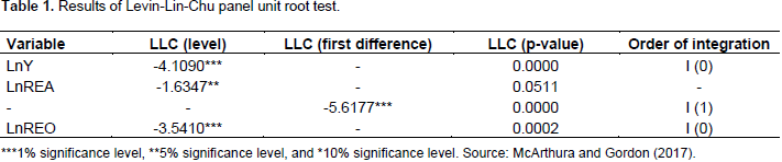
Levin-Lin-Chu panel unit root test was used to conduct stationarity test and it is based on the following hypotheses:
Ho: Each time series contains a unit root HA: Each time series is stationary From Table 1, agricultural output growth and R&D in other sectors were found to be stationary at level and statistically significant at 1% level while agricultural R&D was found to be non-stationary at level but became stationary after first differencing that is integrated of order one and this was statistically significant at 1% level. Co-integration refers to the long run linear relationship of two variables that are stationary after differencing and have to be integrated of the same order. Usually after differentiating, variables tend to lose long run relationship and so co-integration test is being conducted to establish whether variables have got long run relationship after differencing. Since the dependent variable (agricultural output growth) was found to be stationary at level, conducting co-integration test was impossible because the dependent variable and all the independent variables were now not integrated of the same order.
Hausman test was conducted was conducted to establish whether to use fixed effect or random effect regression model and it is based on the following hypotheses:
HO: Preferred model is random effects model
HA: Preferred model is fixed effects model
From the Hausman test in Table 2, the p-value is greater than 0.05 which means that the difference is not statistically significant and so the null hypothesis of the preferred model being random effects model was not rejected. So the random effects regression model was used to analyse the relationship between the dependent variable and the independent variables. Random effects regression was therefore carried out and the results were as per the Table 3. From the results in Table 3, the within R squared is 0.5628. This means that 56.28% of the variations on the agricultural sector growth (dependent variable) within the individual countries are explained by the explanatory variables in the model. The between R squared is 0.5012. This means that 50.12% of the variations on the agricultural sector growth between the entities (countries of the EAC) are explained by the explanatory variables in the model. The overall R squared is 0.5820. This means that 58.20% of the changes on the dependent variable (agricultural output) in EAC are explained by the explanatory variables that are included in the model.

The constant is 2.9750. This means that without the variables like agricultural R&D expenditure, R&D expenditure in other sectors, the agricultural output growth remains at the level of 2.9750. The p-value is 0.627 and being that the p-value is greater than 0.05, this implies that the constant is not statistically significant at 10% level. From the regression results, the coefficient of agricultural R&D (REA) is 0.8533. This means that a 1% increase in agricultural R&D leads to 0.8533% increase in agricultural output (growth). Since the p-value (0.032) is less than 0.05, it means that the 0.8533% increase in agricultural output is statistically significant at 5% level. The coefficient is positive and this conforms to economic theory. The endogenous growth theory says that R&D leads to increase in the stock of knowledge which in turn has got spill over effects hence leads to economic growth.
This positive relationship could be because allocating funds for agricultural research leads to increased agricultural research which causes increased knowledge about high yielding crops, the invention of drought resistant crops which helped in preventing crop failures in the event of a drought, better ways of improving soil fertility which leads to increased yields, introduction of advanced machines in production which made the production process to go faster, hence, high quality and quantity of products within a short period of time. These advanced machines may include machines for tilling land like tractors, milking machines, harvesting machines and planting machines. Agricultural research and development could have also led to the discovery of crop and livestock diseases, what causes them, how they can be prevented and even a solution should they occur. This boosts crop productivity and hence increased agricultural growth.
Through agricultural research and development, better preservation and storage measures and facilities of agricultural products could have been invented and this helps to reduce post-harvest losses by the farmers hence leading to increased agricultural productivity. Agricultural research also leads to better planting and farming methods which increased agricultural productivity. In addition, agricultural research and development leads to high quality breeds of animals like dairy cows, goats, sheep, and in poultry that are highly productive in terms of milk production, meat and eggs hence leading to increased agricultural output. Improved marketing services also arise as a result of agricultural research and development which further leads to improved agricultural productivity. Once agricultural research and development has been done by a particular research institution or university or an individual and a new product or service is invented, spill over effects of the new knowledge occur and this leads to increased agricultural productivity.
The positive and significant effect of agricultural R&D expenditure could have been as a result of proper dissemination of knowledge generated through agricultural R&D. The finding on the effect of agricultural R&D on agricultural sector growth has coincided with the finding of Fuglie and Maeder (2015) who studied the effect of the adoption of improved crop varieties of 20 crops from 1970 to 2010 that covered 37 sub-Saharan African countries and they found that the improved varieties had a major positive impact on productivity growth and hence the finding was therefore similar to the finding of this study. A similar finding was also made by Rao et al. (2016) whom in their meta-analysis of 2829 specific estimates of returns to agricultural research and development programs and projects in 78 countries found that returns to research had not declined over time and that developing countries generally had higher rates of return (median of 41%) than developed countries (median of 34%).
Lastly, the finding for this study is also similar to the finding of Pardey et al. (2016) who in their analysis on the estimates of returns to agricultural research and development in 25 countries in Africa from 1975 to 2014 found high rates of return to agricultural research and development with a median 35% and mean of 42%. All these findings showed that agricultural R&D or agricultural R&D spending had positive effects on the agricultural sector hence they are similar to the finding of this study. This therefore means that agricultural R&D funding should be increased every financial year to facilitate agricultural R&D. In addition, more agricultural research scientist should be trained and employed for serious agricultural research to be carried out. The coefficient of research and development in other sectors (REO) is 0.3160. This means that 1% increase in R&D in other sectors leads to a 0.3160% increases in the agricultural sector growth (output). The coefficient is positive and statistically significant at 1% level. This result has also conformed to theory and the positive influence can be attributed to the spillover effects of R&D.
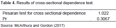
The finding on the effect of research and development in other sectors on agricultural sector growth in the East African Community has coincided with the finding of Rada and Schimelpfenig (2015) that conducted a study on the determinants of total factor productivity growth in India and found that public research made major contributions to total factor productivity growth. Inekwe (2014) who studied the effect of research and development expenditure on economic growth in some developing countries found that research and development expenditure had a positive significant effect on economic growth in countries with higher and medium income levels. His finding was also therefore similar to the finding of this study. So research and development in other sectors is important to the agricultural sector also. Cross sectional dependence is the inter-dependence between cross sectional units. Pesaran and Toseti (2011) test was used to test for cross sectional dependence with the hypotheses stating as follows:
Ho: There exists no correlation of variables across entities
HA: There exists correlation of residuals across entities
From the results of Pesaran’s test for cross sectional dependence in Table 4, the P-value is greater than 0.05 hence the null hypothesis of cross sectional independence was accepted. This means that there was cross sectional independence in the regression analysis. This means that there was no efficiency loss for least square estimators and so conventional t-test and F tests that used variance- covariance estimators were valid. Heteroscedasticity refers to a situation whereby the error terms do not have constant variance across observations. Breusch Pagan Langrange Multiplier (1980) test for heteroscedasticity was used to conduct heteroscedasticity test and its hypotheses are as follows:
HO: Variance across observations is constant
HA: Variance across observations is not constant
From the results in Table 5, the p-value is greater than 0.05 and so the null hypothesis of constant variance was not rejected. This means that heteroscedasticity was not a problem in the regression analysis. This means that the standard errors were unbiased and so there was unbiasness in test statistics and confidence intervals. Autocorrelation is caused by correlation between error terms of different time periods. Autocorrelation in linear panel models causes biased standard errors and makes the estimators less efficient. Wooldridge (2002) test for autocorrelation was used to test for autocorrelation with the hypotheses stating as follows:
HO: There is absence of first order autocorrelation
HA: There is presence of first order autocorrelation
From the results in Table 6, the p-value is greater than 0.05 and so the null hypothesis of no serial correlation was not rejected. This means that autocorrelation was not a problem in the regression results. This means that the standard errors were unbiased and so the estimators were efficient.
CONCLUSION AND RECOMMENDATIONS
The positive and statistically significant relationship between agricultural R&D expenditure and agricultural sector growth could be because of the spillover effects of agricultural knowledge generated through agricultural R&D. This finding coincided with the findings of Fuglie and Marder (2015), Rao et al. (2016), and Pardey et al. (2016) who found that agricultural R&D expenditure or agricultural R&D leads to agricultural sector growth in the various regions and periods that they conducted their studies. In addition, the positive and statistically significant relationship between R&D in other sectors and agricultural sector growth is also being attributed to the spillover effects of R&D. This has also coincided with the findings of Rada and Schimelpfenig (2015) and Inekwe (2014). Based on the results of this study, agricultural R&D and R&D in other sectors influenced agricultural sector growth positively and the influences were statistically significant and to enhance the influences, the following should be done so as to maintain the positive and significant effect of agricultural R&D expenditure and R&D in other sectors.
The government of EAC states to increase the budgetary allocations to agricultural R&D and R&D in other sectors possibly every fiscal year so that more and serious agricultural research and research in other sectors can be undertaken. More agricultural research scientists and research scientists in other disciplines be employed, trained and educated by the government to facilitate serious agricultural research and research in other sectors that can lead to more discoveries on agriculture and also in other fields. That employment terms and conditions to be made favourable to agricultural research scientists and research scientists in other sectors in terms of remunerations and job security so as to motivate them put more effort in their work. The governments of EAC states should ensure that the knowledge generated through agricultural research and research in other sectors is disseminated to the public by employing more agricultural extension officers so as to increase the spill over effects of the knowledge generated through farmers’ education and also through publications in referred journals.
Intellectual property rights need to be enhanced through patents, copyrights and trademarks so as to encourage firms producing agricultural products and inputs to carry out agricultural research, and also to spend more on agricultural research. Lastly, the EAC governments should ensure that more agricultural research institutions and stations are established to increase the intensity of agricultural R&D. The same should also apply to the ones of the other sectors. Based on this study, the scope was limited and other studies can increase sample size and consider other study areas. In addition, future studies can also consider disaggregating agricultural research and development into private agricultural research and development and public agricultural research and development and the same to be done also to other sectors.
The authors have not declared any conflict of interests.
REFERENCES
|
Aghion P, Howwit P (1992). A Model of growth through creative destruction. Econometrica 2(60):323-351.
Crossref
|
|
|
|
Bozkurt C (2015). R&D expenditure and economic growth relationship. Int. J. Econ. Fin. Iss. 5(1):188-198.
|
|
|
|
|
Breusch T, Pagan A (1980). The langrange multiplier test and its applications to model specification in econometrics. Rev. Econ. Stud. 47:239-253.
Crossref
|
|
|
|
|
Bronzini R, Paolo P (2006). Determinants of long-run regional productivity with geographical spillovers: The role of R&D, human capital and public infrastructure. Reg. Sci. Urban Econ. 2(39):187-199.
|
|
|
|
|
Callon M (1994). Is science a public good? Sci. Technol. Hum. Values 19:345-424.
|
|
|
|
|
Cohen W, Levinthal D (1989). Innovation and learning: The two Faces of R&D. Econ. J. 99:569-596.
Crossref
|
|
|
|
|
Cororaton CB (1999). Research and development: A review of literature. Philippine Institute for Development Studies. Discuss. Paper Ser. 99(25):1-63.
|
|
|
|
|
Fuglie K, Marder J (2015). The diffusion and impact of improved food crop varieties in sub-saharan Africa: Crop improvement, adoption and impact of improved varietis in food crops in sub- saharan Africa. CABI. CAB eBooks, Ebooks on agriculture and the applied life sciences from CAB International 17:338.
|
|
|
|
|
Geroski P (1995). Do spillovers undermine the incentive to innovate? Econ. Approach. Innov. 2(3):76-97.
|
|
|
|
|
Grossman GM, Helpman E (1991). Innovation and growth in the economy. MIT press, Cambridge, MA.
|
|
|
|
|
Gisore N, Kiprop S, Kalio A, Babu J (2014). Effect of government expenditure on economic growth in East Africa: A disaggregated model. Eur. J. Bus. Soc. Sci. 3(8):289-304.
|
|
|
|
|
Hausman J (1978). Specification tests in econometrics. Econometrica 46:1251-1271.
Crossref
|
|
|
|
|
Inekwe JN (2014). The contribution of R&D expenditure to economic growth in developing countries. Soc. Indic. Res. pp. 1-19.
|
|
|
|
|
Jones C (2004). Growth and ideas. Handbook Econ. Growth 3(1):1063-1111.
Crossref
|
|
|
|
|
Kadir T, Emir K, Hakan B (2015). The relationship between research and development expenditures and economic growth: The case of Turkey. World conference on Technology, Innovation and Entrepreneurship. Procedia – Soc. Behav. Sci. 195(3):501-507.
|
|
|
|
|
Kim L (2011). The economic growth effect of R&D activity in Korea. Korea World Econ. 1(12):25-44.
|
|
|
|
|
King M, Robson M (1989). Taxation and investment in a dynamic economy. University of Rochester: Mimeo.
|
|
|
|
|
Levin A, Lin C, Chu C (2002). Unit root tests in panel data: Asymptotic and finite-sample properties. J. Econ. 108:1-24.
Crossref
|
|
|
|
|
Mansfield E (1981). Imitation costs and patents: An empirical study. Econ. J. 91:907-918.
Crossref
|
|
|
|
|
McArthura J, Gordon C (2017). Fertilizing growth: Agricultural inputs and their effects in economic development. J. Dev. Econ. 127(1):133-152.
Crossref
|
|
|
|
|
Pardy PG, Andrade RS, Hurley TM (2016). Returns to food and agricultural research and development investments in sub-Saharan Africa (1975-2014). Food Policy 65:1-8.
Crossref
|
|
|
|
|
Pavit K (1999). What makes basic research economically useful? Res. Policy 20:109-119.
Crossref
|
|
|
|
|
Pedroni P (1999). Crucial values for cointegration tests in heterogenous panels with multiple regressors. Oxf. Bull. Econ. Stat. 61:653-670.
Crossref
|
|
|
|
|
Pesaran MH, Toseti E (2011). Weak and strong cross-sectional dependence and estimation of large panels. Econom. J. 14:45-90.
Crossref
|
|
|
|
|
Porter ME (1990). The competitive advantage of nations. Free Press, London.
Crossref
|
|
|
|
|
Rada N, Schimmelpfenig D (2015). Propellers of Agricultural Productivity in India, ERR-203, U.S. Department of Agriculture, Economic Research Service.
|
|
|
|
|
Romer P (1986). Increasing returns and long run growth. J. Polit. Econ. 94:102-37.
Crossref
|
|
|
|
|
Romer P (1990). Endogenous technological change. J. Polit. Econ. 98:71-102.
Crossref
|
|
|
|
|
Rosenberg N (1990). Why do firms do basic research (with their own money). Res. Policy 19:165-174.
Crossref
|
|
|
|
|
Sadraoui T, Ali T, Deguachi B (2014). Economic growth and international R&D cooperation: A panel granger causality analysis. Int. J. Econom. Fin. Manage. 1(2):7-21.
|
|
|
|
|
Scott MFG (1989). A new view of economic growth. Clarendon: Oxford.
|
|
|
|
|
Sheshinski E (1967). Optimal accumulation with learning by doing. In Shell K., (ed.), essays on the theory of optimal economic growth MIT Press: London. pp. 47-58.
|
|
|
|
|
Solow RM (1956). A contribution to the theory of economic growth. Q. J. Econ. 70(1):65-94.
Crossref
|
|
|
|
|
Svensson R (2008). Growth through research and development. Swedish Government Agency for Innovation Systems Report.
|
|
|
|
|
Swan TW (1956). Economic growth and capital accumulation. Econ. Record 32(63):334-361.
Crossref
|
|
|
|
|
Tumushabe G, Mugabe J (2012). Governance of science, technology and innovation in the East African community: Inaugural biannual report. ACODE Policy Res. Series 51:2012.
|
|
|
|
|
Wooldridge J (2002). Econometric analysis of cross section and panel data, 2nd edition. The MIT Press: London.
|
|