ABSTRACT
This study presents an application of the Ricardian approach to explore the impact of climate change on farmland values in Nepal. The Ricardian approach is estimated using a panel fixed effects model, and the outcome is compared against two separate models that account for spatial correlation: a spatial autoregressive (SAR) model; and a spatial error model (SEM). The findings suggest that Nepalese farmlands are sensitive to climate change, and this result was consistent in both the non-spatial and the spatial frameworks. The inclusion of the spatial effects, however, revealed the presence of positive spatial autocorrelation and produced conservative estimates of climate change impacts. The net effect of annual increases in average temperature was negative; while the net effect of higher annual average precipitation was a positive outcome on farmland values. In particular, we found that the marginal effect of every degree increase in average annual temperature was Rs.180 /hectare ($1.80) reduction in farmland values. Likewise, for rainfall, it was found that 1 mm increase in average annual rainfall would positively affect farmland value by Rs.225/hectare ($2.25). Finally, the study findings suggested that extreme weather events could also impact the agricultural productivity and the farmland values in Nepal.
Key words: Climate change, ricardian approach, spatial panel data analysis, Nepalese agriculture, environmental valuation.
Climate change is emerging as a significant threat facing the humanity in the 21st century. There is a consensus among researchers that variations in land and water regimes through changes in climate might pose a significant challenge to the natural and human systems (Intergovernmental Panel on Climate Change (IPCC), 2007, 2014).
Agriculture is one area that is highly sensitive to climate due to its reliance on weather patterns and climate cycles for productivity. Agriculture is also the principal use of land globally with approximately 1.2 to 1.5 billion hectares of lands under crops, while another 3.5 billion hectares are used for grazing (Howden et al., 2007).
One country that is predominantly dependent on agriculture is Nepal. Nepal is a tiny developing country located in South Asia between India and China. The Nepalese agricultural sector contributes to more than one-third to the gross domestic product (GDP), and employs more than half of the total labor force (Acharya and Bhatta, 2013). This notable dependence on agriculture makes the Nepalese farming population highly vulnerable to the impacts of climate change.
Past studies suggest that the average annual mean temperature in Nepal has increased at an annual rate of 0.06°C between 1977 and 2000 (Malla, 2009). It has subsequently led to changes in the frequency of temperature extremes with more frequent warmer days and nights; and less frequent colder days and nights (Gum et al., 2009). Precipitation, on the other hand, has not displayed any definitive trends, but evidence indicates an increasing occurrence of intense rainfall events and rising flood days over the years (Gum et al., 2009). Such instances of extreme weather events can result in desirable agricultural land being undesirable as crop yields are restricted.
These changing climatic conditions have led to shifts in cropping patterns and the agricultural sector in Nepal is consequently being severely hurt. Regmi (2007) indicated that the eastern region of Nepal faced rain deficit in 2005/06, and the crop production was reduced by 12.5% on a national basis. Likewise, while Nepal used to be rice exporter in the past, the fluctuating climate conditions has limited the rice yields, and as a result, Nepal has been a rice importer for the past few years.
Nepal’s heavy dependence on rain-fed agriculture coupled with the potential distressing effect of climate change, and ultimately on the welfare of the population and the economy of the country itself, necessitates a thorough analysis on the economic impact of climate change on the agricultural sector. An exhaustive assessment of the economic impact would allow for new policy formulation on potential mitigation and adaptation strategies to combat the likely effects of climate change. In this paper, an application of the Ricardian approach is used to evaluate the economic impact of climate change on agricultural productivity in rural Nepal.
The Ricardian approach is a model of climate-land value relationship, which was developed by Mendelsohn et al. (1994) to assess the impact of climate change on farmland values in the United States. The Ricardian Method is, in fact, named after the influential classical economist David Ricardo (1772 to 1823), who argued that in a perfectly competitive market, land values would reflect land profitability.
In their paper, Mendelsohn et al. (1994) evaluated the efficacy of the traditional production function approach in estimating the impacts of climate change with a new method they developed, the ‘Ricardian Method’. The production function approach is based on crop simulation models where the climate change impacts are estimated by varying input variables, including the climate itself. Mendelsohn et al. (1994) suggested that the limitation of the production-function approach in failing to account for the numerous substitutions and adaptations that farmers make could lead to an inherent bias that results in an overestimation of the damages from climate change.
The fundamental idea of the Ricardian approach is that land values and agricultural practices are correlated with an environmental variable, climate. However, some assumptions underlie this framework. The Ricardian model assumes that farmers are rational utility maximizers, and relies on an existence of a competitive economy with perfectly functioning output and input markets. With these assumptions, the Ricardian framework asserts that if the optimal use of farmlands is agricultural production, then the observed market rent on a parcel of land should equal the annual net profits from the production of an agricultural commodity using that land (Mendelsohn et al., 1994). Thus, farmland values are the discounted value of current and future profit. Furthermore, we can observe the relationship between farm values to climate and other variables to infer the optimal use of land. Hence, depending on the positive and negative impact of climate variables, the long-run accumulation of net profit defines land value.
Although the Ricardian method has since garnered widespread attention, there have been some notable criticisms as well because of the strong assumptions it makes (Cline, 1996; Darwin, 1999; Polsky, 2004; Deschenes and Greenstone, 2007). Darwin (1999) maintained irrigation to be an essential variable and omitting it would make the model of Mendelsohn et al. (1994) inconsistent with the Ricardian principle. Cline (1996) argued that the assumption of fixed relative prices in the Ricardian approach makes it a partial-equilibrium analysis. Besides, Cline (1996) also contended that the assumption of infinitely elastic supply of irrigation at current prices is misleading. Polsky (2004) argued that because Ricardian models are strongly aligned with perfect adaptations assumption, the negative impacts are biased to be small. Deschenes and Greenstone (2007) raised doubt on the validity of cross-sectional approaches to Ricardian study and proposed the use of a fixed-effect modeling to get more stable results from the Ricardian function.
To incorporate the limitations in the ergodic assumption of spatially and temporally invariant climate sensitivities, Polsky (2004) modeled a modified regional scale Ricardian analysis by integrating spatial and temporal variations in climate. The author reasoned that ignoring spatial relationship (inter-farmer communications across county borders) to understand climate-land use relationship could not account for climatic effects in different locations or time. Following Polsky (2004) there have been few other studies that have explored the Ricardian approach by explicitly incorporating spatial correlation.
Lippert et al. (2009) accounted for spatial auto-correlation in their analysis of the Ricardian approach in German agriculture by using a spatial lag and a spatial error dependence model. Kumar (2011) studied the impact of climate change on Indian agriculture by addressing the spatial features that could influence the climate sensitivity of agriculture. The paper argued that ignoring the spatial distribution could result in enlarged estimates of climate impacts in Ricardian studies. Their estimates of climate change impacts were more conservative after incorporating spatial correction models, and this finding was consistent in both the spatial lag and the spatial error model specification. Other researchers that have explicitly treated the spatial problem in the Ricardian study are Schlenker et al. (2005) and Chatzopoulos and Lippert (2016).
A separate limitation of numerous Ricardian studies that estimate climate change – land value relationships has been with the use of cross-section data for analysis. Since climate coefficients change over time, analyzing farms’ long-term changes using cross-section data may not give reliable estimates. A panel-data approach can be far superior for estimation of any hedonic models, including Ricardian analysis if panel data are available and the time varying and unvarying coefficients are correctly specified (Massetti and Mendelsohn, 2011). A panel data approach also removes year effects and can produce more reliable estimates of the climate coefficients (DeSalvo et al., 2014). Several authors (Massetti and Mendelsohn, 2011; Deschenes and Greenestone, 2011; Massetti et al., 2013), etc. have employed panel data methods to study Ricardian analysis and the trend is rising.
Finally, another issue in many Ricardian studies stems from the use of only historical averages for temperature and precipitation to assess the impact of climate change on agriculture. However, plant physiology literature argues that it is not only the average weather patterns but also the extreme weather events that could have a severe effect on crop yields and agriculture in general (Rosenzweig et al., 2001; Anyamba et al., 2014).
Through this study, we seek to address the research gaps that have been identified in Ricardian analyses, in particular, the concerns mentioned earlier. First, considering the limitations of cross-sectional data approaches in other Ricardian studies, this paper uses panel data approach to enhance estimates reliability. Second, our analysis includes additional climate variables other than seasonal averages that could potentially capture the extremities in climate. Finally, we address the importance of accounting for spatial features and our estimation strategy thereby incorporates spatial methods in the Ricardian approach. Many Ricardian studies ignore the problem of spatial correlation, but when observations are correlated across space, standard approach such as the Ordinary Least Squares (OLS) method can lead to biased and inefficient parameter estimates (LeSage and Pace, 2009). The primary contribution of this paper that separate it from previous Ricardian applications is that we include extreme climate variables, while also explicitly accounting for spatial correlation in a panel data setting to study climate change impacts on agricultural productivity in rural Nepal.
The non-climatic data used in this paper comes from the Nepal Living Standard Survey 2003/04 (NLSS-II) and 2010/2011 (NLSS-III) of the Central Bureau of Statistics (CBS), Nepal. The NLSS survey follows the Living Standards Measurement Survey (LSMS) methodology that has been developed and promoted by the World Bank.
The methodology applied in the NLSS has been used in more than 50 developing countries by the World Bank with the goal to foster increased use of household data as a basis for policymaking. The NLSS survey includes a broad range of topics related to household and community welfare, but the important socio-economic variables necessary for this paper were obtained from the rural community questionnaire of NLSS. As such, this paper focuses on the rural farming communities in Nepal. The rural community questionnaire of the NLSS was developed to interview leaders and knowledgeable persons representing the community of the enumeration areas (CBS, 2004).
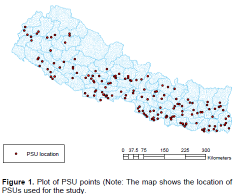
In this study, the primary sampling units (PSUs) are used as the unit of analysis, and not the individual households. The geocoded coordinates were made available only for PSUs, but not for the households, which constrained us to use PSU level analysis to explore the spatial relationship in our study. The total sample of the NLSS-II consists of 4,008 households representing 334 PSUs, from which 100 PSUs were common in NLSS-III as well (CBS,2004). The total sample of the NLSS-III was estimated at 7200 households in 600 PSUs (CBS,2010). Among them, the NLSS-III sample is composed of all households visited by the NLSS-II in 100 of its PSU, as mentioned earlier. The final sample selected from NLSS-II and NLSS-III was 155 PSUs for this study. Figure 1 plots the PSU locations used in this study.
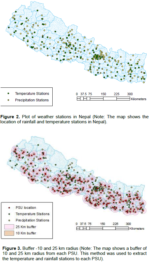
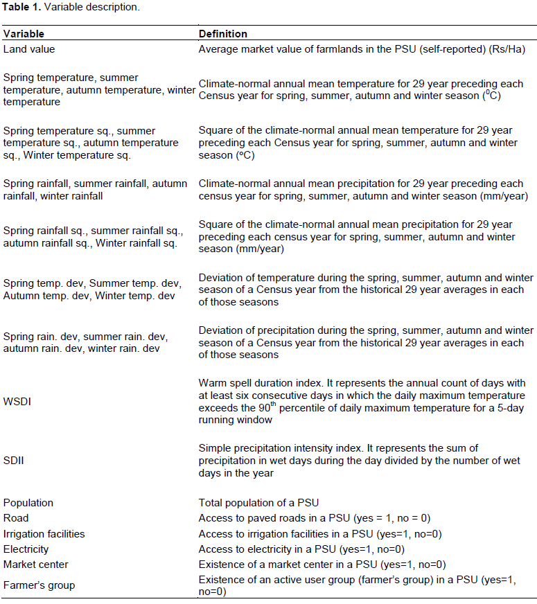
In addition to the community welfare data from NLSS, this study used the ground station climate data for daily temperature and precipitation from 1981 to 2010, obtained from the Department of Hydrology and Meteorology, Nepal. The selection of weather stations nearest to each PSU was made in ArcGIS using multiple buffer width of 10 and 25 km radii. Figure 2 shows the graph of the weather stations in Nepal, and Figure 3 presents the graph of buffer analysis undertaken to extract the weather stations nearest to each PSU. Similarly, Table 1 lists the definition of variables used in this study.
Dependent variable
We used the self-reported average farmland value in each PSU as the measure of net productivity. These values have been converted to a per hectare land value in our analysis. While Ricardian papers often use net revenue or net profits as a proxy for land values, we used the actual farmland value in each PSU, since it was already available in the survey.
A criticism of using net revenue is that it is strongly influenced by the year of analysis (DeSalvo et al., 2014). Land values could be more accurate and an appropriate measure to analyze climate impacts since they reflect the expectations of net revenues across many years (Mendelsohn et al., 2009).
Explanatory variables
Climate variables
In order to construct the climatic variables, the daily temperature, and precipitation data for the time period 1981 to 2010 are used. Temperature and precipitation were classified into four seasons: spring, summer, autumn and winter. We converted the daily average temperature and precipitation data into the four seasonal averages. In order to get the climatic data for 2002, the seasonal average from 1981 to 2002 was taken, and likewise, the seasonal average from 1989 to 2010 was used to capture the 2010 values. The 2002 and 2010 climate data, thus, capture the rolling average for the past 22 years. Using the constructed seasonal averages, the first set of climate variables used were the linear and quadratic measures of seasonal temperature and rainfall. The quadratic variables were introduced to capture the possible nonlinearities in the climate sensitivities.
Along with the seasonal averages, we constructed variables to capture climatic deviations, and also climate extremes. The motivation for the inclusion of variables to capture climate extremities comes from the plant physiology literature that argue frequency and intensity of extreme weather events could also have a significant effect on crop yields and agriculture (Rosenzweig et al., 2001; Anyamba et al., 2014). To capture the climatic variation, we constructed the deviation of the seasonal temperature and precipitation for the year 2002 and 2010, from the rolling average of
the past 29 years, for each of the four seasons.
The other set of climatic variables were employed to capture the extremities in climate, namely, the warm spell duration index (WSDI) for temperature, and simple precipitation intensity index (SDII) for rainfall. These indices are two of twenty-seven indices that have been recommended to assess extreme weather events by the World Meteorological Commission for Climatology/ World Climate Research Program (CCI/CLIVAR) expert team on climate change detection, monitoring and indices through the CLIMDEX project (www.climdex.org). WSDI represents the annual count of days in each year that is part of a warm spell. More specifically, it represents the annual count of days with at least six consecutive days in which the daily maximum temperature exceeds the 90th percentile of daily maximum temperature for a 5-day running window (Bronaugh, 2015). SDII, on the other hand, represents the sum of precipitation in wet days during the day divided by the number of wet days in the year (Bronaugh, 2015).
Non-climatic variables
The set of control variables used in this paper are access to irrigation facilities, access to a market center, access to a road network, access to electricity; and the presence of farmers group, all within the context of the PSUs. Access to irrigation captures whether the PSU has irrigation facilities available. Access to market center means if the PSU has a market center in that community. Access to road and electricity follow similar explanation as for the case of irrigation and market center. Lastly, farmers group captures the existence of user group in a community (Table 2).
Conceptual framework
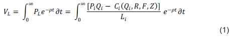
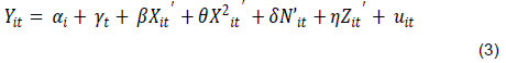
In a Ricardian model, farm performance (land value or net revenue) is regressed on a set of agro-climatic and socio-economic variables to assess the impact of climate change on farm performance. Mendelsohn et al. (1994) argued that the traditional approach to measuring the impacts of climate change on agriculture, the production function approach, was a crop specific analysis and it could overestimate the impacts. To overcome this limitation, the Ricardian approach was developed, and it assumes the following specification (Mendelsohn et al., 1994):
Where, farmland value ( ) reflects the present value land (L); is the net revenue per hectare; and are the market price and output of the crop i respectively; is a function of purchased inputs (excluding land); R is a vector of input prices; F is a vector of climatic variables; Z is a vector of socioeconomic variables; t is the time, and is the discount rate.
The Ricardian model assumes that a farmer will maximize his land value (or net revenue) by choosing inputs subject to climate
(F) and socio-economic variables (Z). This model relies on a quadratic formulation of climatic variables and is presented as:
Where, is an error term. The linear and a quadratic term for temperature and precipitation accounts for the nonlinear shape of the net revenue of the climate response function.
In the study analysis, we regressed the farmland value per hectare in the rural communities of Nepal as a dependent variable against climate and socio-economic variables. The independent climatic variables included the linear and quadratic temperature and precipitation for the four seasons: winter (the average for December, January, and February), spring (March, April, and May), summer (June, July, and August) and autumn (September, October, and November). In addition to the seasonal averages, the study analysis included seasonal temperature and precipitation deviation from the historical 22 years’ seasonal average.
Finally, we incorporated WSDI to measure the temperature extreme, and simple precipitation intensity index (SDII) to measure the rainfall extreme. The independent non-climatic variables include the existence of paved road in the PSU, population of the PSU, whether the PSU had irrigation facilities available, having electricity in the PSU, and the existence of market center and farmers group in the PSU.
Analytical framework
Panel fixed effects (Non-spatial model)
The analytical framework was carried out using a forward specification analysis. First, a panel fixed effects model was run, and the results were compared with a spatial lag and a spatial error model. The general specification of the non-spatial fixed effects model is given by:
The subscripts i and t in equation (3) denote PSU and time, respectively. The dependent variable Y is the farmland value per hectare, and represents the PSU fixed effects. It is assumed that the PSU fixed effects absorb all the unobserved PSU specific time-invariant factors such as soil and water quality that could influence the crop yields and land values. represents the time fixed effects, and it is presumed to control for time differences in the dependent variable which are common across PSU. The variable X is a vector of climate normals; while N captures the vector of climate deviations and extremes. Finally, Z is a vector of PSU sociodemographic variables; and is an idiosyncratic error term that is assumed to be independent and identically distributed over PSUs and time, with mean zero and variance . The fixed effects model concentrates on differences within PSU’s. Thus, it explains to what extent farmland values deviate from average PSU farmland value.
While the parameter estimates from equation (3) could provide evidence on the impact of climate change on farmland values in Nepal, the estimates could be biased if land values are spatially correlated. In fact, Tobler (1979) first law of geography states that ‘near things’ are more related than ‘distant things’. This suggests that farmland values could be spatially auto-correlated if there is a dependency between farmland prices. In a developing country like Nepal where farmers may not have sufficient information about their land characteristics, it is likely that land values could depend on interactions across PSUs with other land owners. Patton and McErlean (2003) argue interaction among landlords in order to base their starting price may give rise to spatial relationships.
This provides a motivation to reassess our problem by incorporating the spatial framework. Additionally, spatial modeling might also reduce omitted variable bias and account for spatial heterogeneity from a data-driven perspective. Omitted variable can arise because unobservable factors (for example, location amenities, PSU prestige, water accessibility for irrigation, etc.) could influence the dependent variable (farmland values), and this can be accounted by incorporating a spatial error model (LeSage and Pace, 2009). On the other hand, a spatial autoregressive (lag) model would be crucial if we believe that herd behavior exists in farmland markets, that is, the selling price of farmlands at any particular location acts as a signal that guides the selling price of nearby lands.
Spatial models
Taking into account the potential nature of the spatial relationship in farmland markets, the study analytical framework next incorporated spatial correlation in the Ricardian model. A general specification of the related family of the spatial model takes the following form:
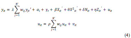
Equation (4) presents the specification of the panel spatial model, and it is similar to the non-spatial fixed effects model detailed in equation (3). The interpretation of parameters ( ) and the variables captured by X, N and Z vectors are same as in equation (3). The additional terms in the spatial model that differentiate it from the non-spatial one are the spatially lagged dependent variable, and the spatial autoregressive process in the error term. The spatial lag coefficient is captured by , while captures the spatial error coefficient. The spatial autoregressive (lag) model (SAR) posits that the dependent variable (farmland value) is influenced by the dependent variables in the adjacent units and on a set of observed local characteristics. The spatial error model (SEM), on the other hand, states that the dependent variable (farmland value) depends on a set of observable characteristics with errors that are correlated across space (Elhorst, 2014).
One of the crucial inputs that spatial models require is the weight matrix W, which summarizes the spatial relations between n spatial units. In particular, the spatial matrix assigns nonzero elements for each observation (row) whose locations (columns) belong to its neighborhood (Anselin and Bera, 1998). A row-standardized weight matrix, where the row of the spatial weight matrix sums to unity, is used in our spatial model. The wy term in equation (4) represents the weighted average of the surrounding observations in the dependent variable; while the wu term represents the weighted average of the surrounding error term. The spatial weight matrix, W, used in this paper is a 5-nearest neighbor weight matrix for the PSUs in our sample. The parameters and measures the extent of the spatial autocorrelation. Furthermore, setting the value of = 0 leads to the SAR model that exhibits relationship only in the dependent variable. Similarly, setting = 0 leads to the SEM, resulting in spatial dependence in only the error term. In the case of the spatial models, the parameters to be estimated are the regression coefficients ; along with the spatial lag coefficient , and the spatial error coefficient, ( .
Marginal impacts
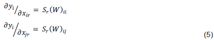
The standard interpretation of estimated parameters as partial derivative is no longer valid in the case of the SAR model. Intuitively, the lag model implies that the farm land values of region i is also influenced by the land values from neighboring regions. The marginal effects in the SAR model take the following form (LeSage and Pace, 2009):
Where, . In equation (5), the subscript i and j represents location i and j respectively, while is the coefficient on the rth explanatory variable. is a n X n matrix with the diagonal elements containing the direct impacts and the off-diagonal elements representing the indirect impacts. In the SAR model, the spatial connectivity relationships mean that a change in a single explanatory variable in region i has a ‘direct impact’ on region i as well as an ‘indirect impact’ on other regions, j i (LeSage and Fischer, 2008).
The upper quantity in equation (5) captures the impact of a change in an explanatory variable (for example, temperature) at location i on the dependent variable at location i, known as the average direct impact (ADI). For example, the average direct effect shows the impact of climate change on PSU i on the farmland values of PSU i. The lower quantity, on the other hand, captures the effect of a change in the explanatory variable at location j on the dependent variable at location i, with j i and is known as the average indirect effect (AII). For example, the average indirect effect, also known as the neighboring effect, measures the impact of an increase in climate at PSU i on the farmland value of neighboring PSUs, averaged over all neighboring PSUs. The average direct effect can be interpreted as the own derivative, while the average indirect effect captures the cross derivative. Lastly, the average total effect (ATI) is the sum of average direct and indirect effect, and it measures the total cumulative impact. In this paper, the average total effects estimate how changes in climate affect total farmland values, taking into account both own-PSU and spillover effects.
Marginal climate impacts
Since the study climate variables contain linear and quadratic coefficients in raw form, we evaluated the marginal climate impacts (MCI) for rainfall and temperature to ease interpretation. Recalling equation (3), the MCI of average annual changes in climate (temperature or precipitation) on the mean farmland value per hectare can be expressed as:
In this study, the MCI represents the change in Rs./ha of farmland value per 0C or mm/year, evaluated at the mean annual climate for farmlands in Nepal.
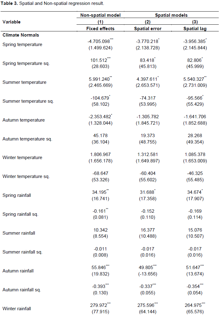
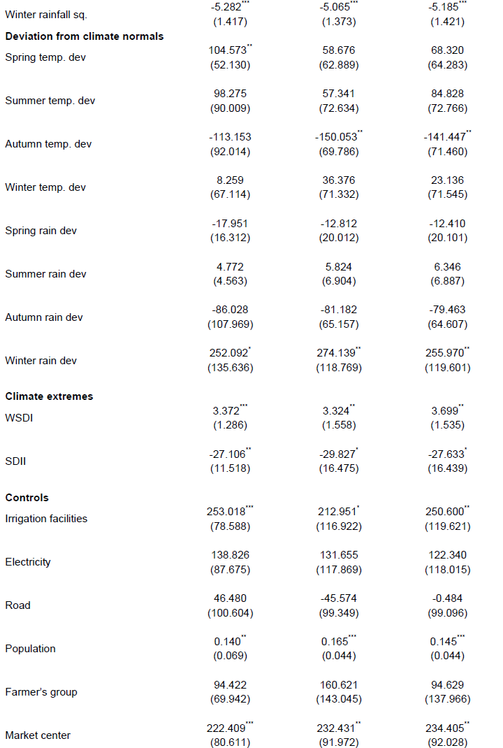
The data summary (Table 2) shows that most of the variables have low standard deviation, indicating data homogeneity. The regression results from the non-spatial fixed effects model (Table 3, Column 1) suggested that the spring and summer temperature; and the spring, autumn and winter rainfall impacted the farmland values. Likewise, the spring temperature deviation and the winter rainfall deviation, as well as the extreme indices in WSDI and SDII also affected the farmland values. The non-climatic variables that were found to be significant were irrigation facilities, population and the existence of market center in the PSU, all of which had a positive impact on the farmland values. The significance of these variables was almost identical in the spatial lag and the spatial error model as well (Table 3, Column 2 and 3).
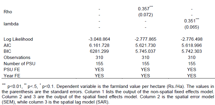
While the significance of most variables were comparable in all three models, the magnitudes of the estimated climate coefficients were smaller in spatial models than the non-spatial fixed effect model. Furthermore, the spatial correlation parameter ( in the spatial error model and the spatial autoregressive parameter ( in the spatial lag model were both significant, suggesting the presence of spatial correlation. The positive coefficient on the spatial lag parameter indicates that farmland values are positively affected by land values in the neighboring PSU’s. This finding substantiates the need to incorporate spatial effects in our modeling, and ignoring these effects to explore the impact of climate change on farmland values can lead to biased estimates. In order to choose the best spatial model, we relied on the lowest AIC and the BIC values (Table 3). While the estimates of the AIC and the BIC values largely favored the spatial models over the non-spatial one, the SAR model was only slightly preferred over the SEM model based on the goodness of fit estimates (Table 3).
We also found evidence that extremities in weather could affect farmland values too. This was revealed by the fact that areas with more warmer days throughout the year had higher farmland values; while areas with more intense precipitation had lower farmland values. Additionally, the climate change impact estimates displayed non-linear relationship with farmland values in certain seasons, and this result is consistent with the Ricardian hypothesis proposed by Mendelsohn et al. (1994).
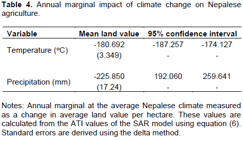
Finally, we looked at the marginal effect of average annual temperature and rainfall changes in farmland values. The net effect of increasing annual temperature was negative; while the net effect of higher annual precipitation was a positive outcome on farmland values (Table 4). In particular, we found that the marginal effect of every degree increase in average annual temperature was Rs.180 /hectare ($1.80) reduction in farmland values. In contrast, every mm increase in annual average rainfall led to an increase in farmland values by Rs.225/hectare ($2.25) (US$1 = Nepali Rs.100 conversion rate of 22 April, 2015 used throughout).
The findings from both, the non-spatial and the spatial models, suggested that climate does seem to have an impact on the value of farms in Nepal. For instance, the non-spatial fixed effect model showed evidence that the average temperature during the spring and summer season; and the average rainfall during the spring, winter and the autumn season affected the farmland values.
Additionally, the presence of a nonlinear relationship between climate and land values, although present only in certain seasons, is consistent with the findings from other Ricardian studies (Mendelsohn et al., 1994; Deressa et al., 2005; Seo and Mendelsohn, 2008). The effect of temperature on farmland value was more pronounced than that of rainfall, and this suggests higher sensitivities of crop growth to temperature changes (Lobell and Burke, 2008). Regarding precipitation, the result indicated that although higher rainfall is conducive for crop development, excess rainfall could hurt the crops, and, thereby the farmland values.
In essence, the significant quadratic variables imply that climate and farmland values have a nonlinear relationship, and it is consistent with the hypothesis of Ricardian approach (Mendelsohn et al., 1994). The positive coefficient in the quadratic terms for temperature (rainfall) suggests a minimally productive level of temperature (rainfall) and either more or less temperature (rainfall) would increase land values. The negative quadratic coefficients for temperature (rainfall) indicate that there is an optimal level of climate variable from which the value function decreases in both directions (Mendelsohn et al., 1994).
The findings from Table 3 shows that the significance of the variables for both the non-spatial (Column 1) and spatial models (Column 2 and 3) was almost alike. While the sign and significance of most coefficients in the three models were comparable, the magnitudes of the climate normal variables in the non-spatial model were larger in absolute value compared to the spatial models. This finding is consistent with other papers that have examined spatial and non-spatial modeling in the context of Ricardian framework (Kumar, 2011; Baylis et al., 2011).
The linear and the quadratic temperature variable for the spring season was significant across all models, while for the summer, the variables were significant in the non-spatial (column 1) and the SAR model (column 3). Winter temperature did not have any effect on farmland values across all three models, while the linear term for the autumn temperature was significant only in the non-spatial model. Looking at column (3), the turning point for spring temperature occurred at 23.88°C. This indicates that average spring temperature above 23.88oC is associated with higher crop yields, which results in higher farmland values as well.
Similarly, the turning point for summer temperature in column (3) is 28.98°C, indicating that farmland values decline when average summer temperature exceeds 29°C. This result makes sense when we consider the major agricultural outputs of Nepal. The major crops grown in Nepal are paddy, wheat, and maize (Malla, 2009); and the optimal temperature range estimated in this paper is consistent with literature that have explored these crop’s life cycle. Karn (2014) found that the critical temperature threshold for rice yield in Nepal to be 29.9°C, and temperature beyond that would lead to a decline in rice yields. Bhatt et al. (2014) found that the critical maximum threshold for maize production to be 27°C in Eastern Nepal. Bannayan et al. (2004) also suggest the optimum temperature for maize growth, in general, should be between 22 to 25°C. These findings could potentially explain the results found in this paper for the decline in farmland values at temperatures below 23.88°C and beyond 28.98°C. Since the suitable temperature for both maize and rice in Nepal lies between about 22 to 30°C, it seems plausible that farmland values increase in that temperature range.
The other significant climatic variables across all three models were the winter rainfall deviation, WSDI, and SDII. In particular, higher rainfall deviation during the winter season; and areas with higher annual warmer spells, both had a positive impact on farmland values. On the other hand, areas with more intense and excessive rainfall, in general, were associated with lower farmland values. Although the winter temperature was not significant in any of the models, we believe that is due to the growth requirement of winter crops in Nepal. The main winter crops in Nepal are wheat and barley, which have been found to be highly sensitive to winter rainfall, moreso than temperature (Krishnamurthy et al., 2013). In fact, Krishnamurthy et al. (2013) state that the winter crops in Nepal are extremely sensitive to small changes in rainfall patterns while the impact of temperature on these crops is low.
The coefficients on the linear and the quadratic precipitation variables suggest that autumn and winter average rainfall affect farmland values and this result is consistent across all three models. Similarly, higher spring precipitation had a significant and positive consequence on farmland values across all three models. This result also seems plausible when we consider the harvesting period of the major crops in Nepal. The harvesting period in Nepal for rice starts from mid-October to December, while wheat is harvested in winter period. Thus, the positive coefficients in the autumn and winter rainfall imply the presence of suitable environment for these crops during harvest time, which is positively reflected on the land values. Likewise, the negative coefficients on the quadratic terms for winter and autumn precipitation imply that excessive rainfall during these seasons could potentially damage the harvest, thereby negatively affecting the land values.
The other findings were that PSU’s with access to irrigation, market center, and with higher population have a positive impact on farmland values. These results also seem reasonable since PSUs with irrigation facilities would not need to rely on rain-fed agriculture for crop growth and thus, these areas have higher land values. Similarly, presence of market center provides opportunities to easily purchase different agricultural products to improve yield; and higher population implies location with better amenities that could be driving population growth, both of which would result in higher farmland values as suggested by the results in this paper. In fact, the positive impact of irrigation facilities and market center on Nepalese farmland valuation has also been confirmed by Joshi et al. (2017).
The findings from the spatial analysis revealed the need to incorporate spatial models to enhance estimation reliability. With regards to the choice between the two spatial models, we looked at the model performance parameters, the AIC, and the BIC values, which suggested SAR as a slightly better model. While the SAR model was preferred from an econometric perspective, this lag model seems probable from an intuitive viewpoint as well. It is reasonable to assume that since farmers may not know the inherent value of their land due to insufficient information about land characteristics, especially in developing countries like Nepal, land prices could thereby depend on landowner interactions across communities.
Similarly, one can also argue that farmlands surrounded by expensive lands could potentially be worth more than those surrounded by inexpensive lands. Additionally, agricultural land markets are highly localized with many buyers being farmers looking to add fields near to their existing operation (Baylis et al., 2011), which further strengthens the argument for the use of the lag model. Anselin et al. (2008) state that for an equilibrium outcome of a spatial or social interaction process where the value of a dependent variable for one agent is jointly determined with that of neighboring agents, a SAR is considered to be ideal.
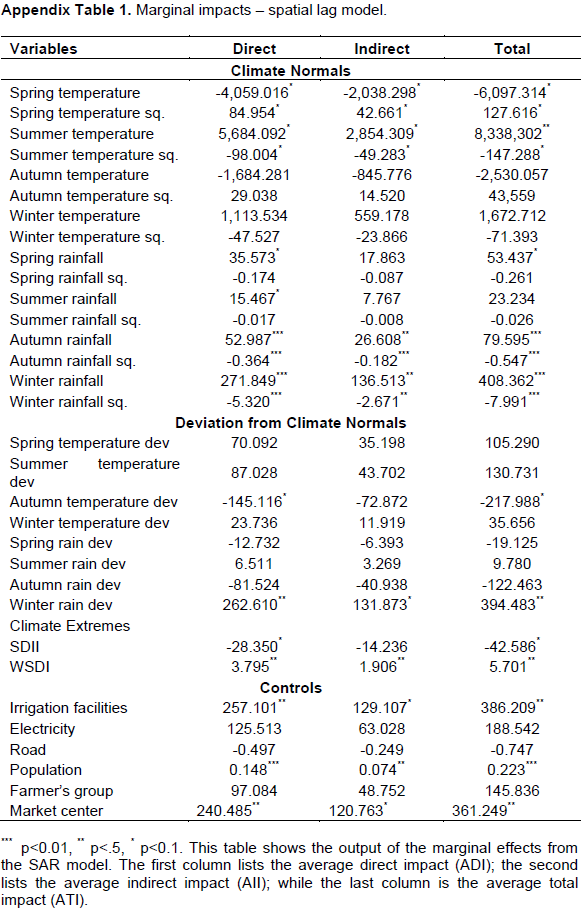
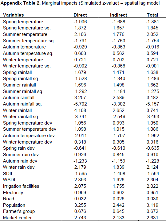
We then looked at the marginal impacts of the SAR model (Appendix Table 1). The direct effect showed that for every degree increase in the spring temperature beyond the threshold value of 23.88°C, farmland values increased by Rs.85/hectare ($0.85). However, beyond 28.98°C temperature in the summer season, every degree increase in temperature reduced farmland values by Rs.98/hectare ($0.98). The average indirect impact for the spring and summer temperature were also significant, indicating that the temperature at a particular PSU also affects the land values of neighboring PSUs (as defined by the W matrix). The indirect effect implied that for every degree increase in spring temperature beyond 23.88°C at a particular PSU, the land values in the neighboring PSUs increased by Rs.42/hectare ($0.42).
Likewise, beyond 28.980 C in the summer, farmland values in the neighboring PSUs declined by Rs.49/hectare ($0.49). The significance of the indirect effect does not seem implausible since climate is not vastly dissimilar in a small spatial scale. Therefore, if spring temperature affects the land values at a particular PSU, it is likely to affect the neighboring PSUs as well. Finally, the average total impact of an increase in the spring temperature beyond 23.88°C suggested that for every degree increase, the total farmland value increased by Rs.127/hectare ($1.27), when taking into account the own-PSU effect and the spillover effect of a change in spring temperature. The impact of summer temperature on farmland values can be interpreted in a similar fashion. Taking into account the findings from changes in temperature, the overall net marginal effect of a degree increase in average annual temperature was a reduction in farmland values by Rs.180/hectare ($1.80) (Table 4).
Regarding rainfall, the findings suggested that the average direct impact of a mm increase in rainfall during the spring season increased farmland values by Rs.35/hectare ($0.35). Precipitation during autumn and winter season also had an impact on the farmland values. Similar to the case of spring temperature, the average indirect impact indicates that precipitation during these seasons was not only affecting farmland values at that PSU, but also the land values in the neighboring PSUs. The average direct impact of an increase in precipitation during autumn and winter season was Rs.52/hectare ($0.52) and Rs.271/hectare ($2.71) respectively. However, excessive rainfall destroys crops, and it is reflected in the lower land value captured by the negative quadratic terms. Finally, the overall net marginal impact of a mm increase in the annual mean rainfall was an increase in farmland value by Rs.225/hectare ($2.25) (Table 4).
SDII and WSDI, the two variables that capture the extremities in climate were also both significant. Higher SDII suggests the occurrence of stronger precipitation, and this has an adverse impact on farmland values. On the other hand, higher WSDI, which indicates greater number of warmer days, positively affects the farmland values. Heavy rainfall can cause a disruption in crop cycle balance and lead to lower yield which could negatively affect farmland values, as suggested by our findings.
The positive effect of WSDI also makes sense since paddy, one of the major crops in Nepal, requires an extended period of the warm growing season. Similarly, maize is another staple crop of Nepal which also requires warm days to grow properly, and thus higher WSDI can, in fact, lead to higher farmland values. The results for the average total impacts suggested that intense precipitation lowered farmland values by Rs.42.5/hectare ($0.425); while higher days of warm spell increased land value by Rs.5.70/hectare ($0.057). In terms of the non-climatic variables, PSUs with access to irrigation and market center had land values that were higher by Rs.386/hectare ($3.86) and Rs.361/hectare ($3.61) respectively, compared to the ones that did not have those amenities.
Changes in climate and the resulting changes in land use pattern are likely to have a significant impact on sectors like agriculture, forestry, water and food security (Field, 2012). While the severity of climate change impacts on agriculture could be massive, with the right mitigation and adaptation strategies, the negative consequences can be alleviated. This paper used an application of the Ricardian approach to analyze the impact of climate change on farmland values in Nepal. Taking into account the limitation of traditional Ricardian approach in failing to explicitly incorporate the spatial nature of land values, this paper employed a spatial fixed effect model to estimate climate change impacts in the context of Nepal. The results revealed significant evidence of spatial correlation and the effects of climate change were found to be more conservative in spatial models relative to the non-spatial model.
The general findings implied that Nepalese farmlands are sensitive to climate change. The average temperature during the spring and summer season; and average rainfall in the spring, autumn and winter season were found to affect crop yields and thereby, the value of farms. The net effect of annual increases in temperature was negative; while the net impact of higher annual precipitation was a positive outcome on farmland values. In particular, we found that the marginal effect of every degree increase in annual temperature was Rs.180/hectare ($1.80) reduction in farmland values. Likewise, for rainfall, it was found that 1mm increase in average annual rainfall would positively affect farmland value by Rs.225/hectare ($2.25). Additionally, the extreme weather indices suggested PSUs with a greater number of warmer days (WSDI) faced positive effect on farmland values; while PSUs with excessive precipitation (SDII) had lower farmland values.
From a modeling perspective, we found evidence of significant positive spatial correlation, and the aforementioned results are the outcome of a spatial correction model. The implication of our findings from an econometric perspective suggests the need to depart from non-spatial analysis to studies that account for spatial analysis in order to obtain more reliable estimates of climate change impacts on farmland value.
The results from this study also provide an interesting perspective from the policymaking point of view. Agricultural production is one of the major means of livelihood for most people in Nepal and as such, policies should be directed towards helping people combat the impacts of climate change. One solution could be to provide farmers support in the form of loans, access to seeds, and technical advice on crop management and water harvesting so they can better adapt to the changing climatic conditions. The poor farming population are most vulnerable to climate change, particularly because they rely heavily on rain-fed agriculture. As such, policies should be directed towards providing irrigation systems at minimal costs to these populations. Furthermore, policymakers should also provide education and awareness to farmers on the dangers of climate change as well as on the importance of employing irrigation as a way to increase their crop yields and sustain their livelihood.
The authors have not declared any conflict of interests.
REFERENCES
|
Acharya SP, Bhatta GR (2013). Impact of climate change on agricultural growth in Nepal. NRB Econ. Rev. 25(2):1-16. |
|
|
Anyamba A, Small JL, Britch SC, Tucker CJ, Pak EW, Reynolds CA, Crutchfield J, Linthicum KJ (2014). Recent weather extremes and impacts on agricultural production and vector-borne disease outbreak patterns. PLoS One 9(3):e92538.
Crossref |
|
|
|
Anselin L, Bera AK (1998). Spatial dependence in linear regression models with an introduction to spatial econometrics. Statistics Textbooks Monogr. 155:237-290. |
|
|
Anselin L, Le Gallo J, Jayet H (2008). Spatial panel econometrics. In The econometrics of panel data Springer Berlin Heidelberg. pp. 625-660.
Crossref |
|
|
Bannayan M, Hoogenboom G, Crout NMJ (2004). Photothermal impact on maize performance: A simulation approach. Ecol. Model. 180(2):277-290.
Crossref |
|
|
Baylis K, Paulson ND, Piras G (2011). "Spatial approaches to panel data in agricultural economics: a climate change application. J. Agric. Appl. Econ. 43(3):325-338.
Crossref |
|
|
Bhatt D, Maskey S, Babel MS, Uhlenbrook S, Prasad KC (2014). Climate trends and impacts on crop production in the Koshi River basin of Nepal. Reg. Environ. Change 14(4):1291-1301.
Crossref |
|
|
|
Bronaugh D, Hiebert MJ (2015). Pacific Climate Impacts Consortium. climdex.pcic: PCIC Implementation of Climdex Routines [Computer software manual]. Retrived from https://CRAN.R-project.org/package=climdex.pcic (R package version 1.1-6). |
|
|
|
Central Bureau of Statistics (CBS) (2004). Nepal Living Standards Survey: Statistical Report 2003/04, Volumes I and II. Kathmandu: National Planning Commission/ His Majesty's Government of Nepal. |
|
|
|
Central Bureau of Statistics (CBS) (2010). Nepal Living Standards Survey: Statistical Report 2010/11, Volumes I and II. Kathmandu: National Planning Commission/ His Majesty's Government of Nepal. |
|
|
|
Cohen J, Cohen P, West SG, Aiken LS (2013). Applied multiple regression/correlation analysis for the behavioral sciences. Routledge. |
|
|
Chatzopoulos T, Lippert C (2016). Endogenous farm-type selection, endogenous irrigation, and spatial effects in Ricardian models of climate change. Euro. Rev. Agric. Econ. 43(2):217-235.
Crossref |
|
|
|
Cline WR (1996). The impact of global warming of agriculture: comment. Am. Econ. Rev. 86(5):1309-1311. |
|
|
Darwin R (1999). The impact of global warming on agriculture: A Ricardian analysis: Comment. Am. Econ. Rev. 89(4):1049-1052.
Crossref |
|
|
Deressa T, Hassan R, Poonyth D (2005). Measuring the impact of climate change on South African agriculture: the case of sugarcane growing regions. Agrekon 44(4):524-542.
Crossref |
|
|
De Salvo M, Begalli D, Signorello G (2014). The Ricardian analysis twenty years after the original model: Evolution, unresolved issues and empirical problems. J. Dev. Agric. Econ. 6(3):124-131.
Crossref |
|
|
Deschenes O, Greenstone M (2007). The economic impacts of climate change: evidence from agricultural output and random fluctuations in weather. The American Economic Review, 97(1), 354-385.
Crossref |
|
|
Deschenes O, Greenstone M (2011). Using panel data models to estimate the economic impacts of climate change on agriculture. Handbook on Climate Change and Agriculture pp. 112-140.
Crossref |
|
|
Elhorst JP (2014). Spatial panel data models. In Spatial Econometrics. Springer Berlin Heidelberg pp. 37-93.
Crossref |
|
|
Field CB (2012). Managing the risks of extreme events and disasters to advance climate change adaptation: special report of the intergovernmental panel on climate change. Cambridge University Press.
Crossref |
|
|
|
Gum W, Singh PM, Emmett B (2009). Even the Himalayas have stopped smiling': climate change, poverty and adaptation in Nepal. 'Even the Himalayas have stopped smiling': climate change, poverty and adaptation in Nepal. |
|
|
Howden SM, Soussana JF, Tubiello FN, Chhetri N, Dunlop M, Meinke H (2007). Adapting agriculture to climate change. Proceed. Natl. Acad. Sci. 104(50):19691-19696.
Crossref |
|
|
|
IPCC (2007). Climate Change 2007: Synthesis Report. Contribution of Working Groups I, II and III to the Fourth Assessment Report of the Intergovernmental Panel on Climate Change [Core Writing Team, Pachauri, R.K and Reisinger, A. (eds.)]. IPCC, Geneva, Switzerland 104 p. |
|
|
|
IPCC (2014). Climate Change 2014: Synthesis Report. Contribution of Working Groups I, II and III to the Fifth Assessment Report of the Intergovernmental Panel on Climate Change [Core Writing Team, R.K. Pachauri and L.A. Meyer (eds.)]. IPCC, Geneva, Switzerland, 151 pp. |
|
|
Joshi J, Ali M, Berrens RP (2017). Valuing farm access to irrigation in Nepal: A hedonic pricing model. Agric. Water Manage. 181:35-46.
Crossref |
|
|
|
Karn PK (2014). The impact of climate change on rice production in Nepal (No. 85). |
|
|
|
Krishnamurthy PK, Hobbs C, Matthiasen A, Hollema SR, Choularton RJ, Pahari K, Kawabata M (2013). Climate risk and food security in Nepal—analysis of climate impacts on food security and livelihoods.
View
|
|
|
Kumar KK (2011). Climate sensitivity of Indian agriculture: do spatial effects matter?. Cambridge J. Reg. Econ. Soc. P. rsr004.
Crossref |
|
|
LeSage JP, Fischer MM (2008). Spatial growth regressions: model specification, estimation and interpretation. Spatial Econ. Anal. 3(3):275-304.
Crossref |
|
|
LeSage JP, Pace RK (2009). Introduction to Spatial Econometrics (Statistics, textbooks and monographs). CRC Press.
Crossref |
|
|
Lippert C, Krimly T, Aurbacher J (2009). A Ricardian analysis of the impact of climate change on agriculture in Germany. Clim. Change 97(3):593-610.
Crossref |
|
|
Lobell DB, Burke MB (2008). Why are agricultural impacts of climate change so uncertain? The importance of temperature relative to precipitation. Environ. Res. Lett. 3(3):034007.
Crossref |
|
|
Malla G (2009). Climate change and its impact on Nepalese agriculture. J. Agric. Environ. 9:62-71.
Crossref |
|
|
Massetti E, Mendelsohn R (2011). Estimating Ricardian models with panel data. Clim. Change Econ. 2(04):301-319.
Crossref |
|
|
|
Massetti E, Nascimento GRDC, Fortes de Oliveira A, Mendelsohn RO (2013). The Impact of Climate Change on the Brazilian Agriculture: A Ricardian Study at Microregion Level. |
|
|
|
Mendelsohn R, Nordhaus WD, Shaw D (1994). The impact of global warming on agriculture: a Ricardian analysis. Am. Econ. Rev. pp. 753-771. |
|
|
|
Meyers RH (2000). Classical and modern regression with applications (Duxbury Classic). Duxbury Press, Pacific Grove. |
|
|
Patton M, McErlean S (2003). Spatial effects within the agricultural land market in Northern Ireland. J. Agric. Econ. 54(1):35-54.
Crossref |
|
|
Polsky C (2004). Putting space and time in Ricardian climate change impact studies: Agriculture in the US Great Plains, 1969–1992. Ann. Assoc. Am. Geogr. 94(3):549-564.
Crossref |
|
|
Rosenzweig C, Iglesias A, Yang XB, Epstein PR, Chivian E (2001). Climate change and extreme weather events; implications for food production, plant diseases, and pests. Glob. Change Hum. Health 2(2):90-104.
Crossref |
|
|
Schlenker W, Hanemann WM, Fisher AC (2005). Will US agriculture really benefit from global warming? Accounting for irrigation in the hedonic approach. Am. Econ. Rev. 95(1):395-406.
Crossref |
|
|
|
Seo SN, Mendelsohn R (2008). Climate change impacts on Latin American farmland values: the role of farm type. Rev. Econ. Agron. 6(2):159-176. |
|
|
Tobler WR (1979). Cellular geography. In Philosophy in geography. Springer Netherlands pp. 379-386.
Crossref |
APPENDIX