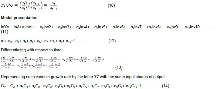
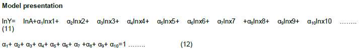
Representing each variable growth rate by the letter ‘G’ with the same input shares of output:
When the growth rate of agricultural output is regressed on the 10 inputs used, the intercept value GA will estimate the average percentage growth in TFP per annum that is growth rate of TFP. When multiplied by 14, the resultant will be TFPG for the entire 15 years.
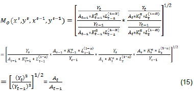
This gives an index of growth or contraction of TFP from year ‘t-1’ to ‘t’ used in GAA procedure. This is the same as in equation 10. According to Fare et al. (1994), this formulation in Equation 15 is equivalent to the more general formulation by Robert Solow (1957), which is the basis for the GAA to measure TFP.
According to Hulten (2000), all the productivity measurement procedures are complementary to one another. In the words of Lovell (1993): “In my judgment neither approach strictly dominates the other, although not everyone agrees with this opinion, there still remains some true believers out there”. In a commentary to this assertion, Kathuria et al. (2013) remarked that no TPFG calculation is superior to the other. The use of any technique depends on the unique situation of the researcher. According to them (Kathuria et al. (2013)), the selection can be based on factors like multiple inputs and outputs, specification of functional form, outliers, sample size, prevalence of high collinearity among inputs, noise, such as measurement error, statistical testing.
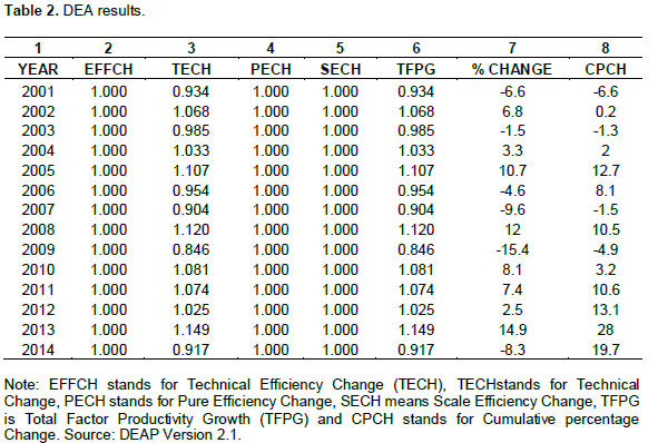
The two procedures (DEAMPI and GAA) does not consider technical efficiency, scale efficiency as well as prices. They are also both non-parametric approaches (Kathuria et al., 2013). As noted by Fare et al. (1994), when technical efficiency is not considered, especially in the single firm case, TFPG will then be synonymous to TECH. In the same vain, the TFPG in the DEA analysis is equal to TECH, because the other two components, EFFCH and SECH are all constants throughout. This clearly seen in the DEAP results in Table 2. It is for this same reason that the A (t) component in the Cobb-Douglas from which Solow proved the GAA, is simultaneously referred to as TECH and TFPG.
Data
The data used for this study are primarily secondary data from six main sources; the Statistics Division of Food and Agriculture Organization of The United Nations (FAOSTAT), International Labor Organization (ILO), The World Bank Development Indicators (WDI), International Fertilizer Association (IFA), the State Hydraulic Works of Turkey (Devlet Su Ä°ÅŸleri-DSÄ°) and the most valuable Turkish Statistical Institute (TUIK). The data covered a period of 15 years spanning from 2000 to 2014. It must be noted that some of the values for some years of some variables were extrapolated, especially for 2014. This was necessary because some of the official values for those variables were not released as at the data collection period.
Variables
The study considered one output and 10 inputs at the aggregate national level. Unlike agricultural output at the farm level, we felt that aggregate agricultural output at the national level requires the inter play of many inputs. The number of input used in studies reviewed ranged from 3 to 6. We recognize the challenges faced in analyzing more variables, especially some software’s inability to deal with more variables. Normally, the data is given the chance to determine which functional form fits it better, however because many inputs are considered, available software are not able to deal with the analysis if it takes a translog production form. Frontier 4.1c, Stata 14 and R 3.0.1 programs could not cope up with the total number of independent variables (regressors) considered for the analysis. In the translog form, the total number of regressors or inputs generated is 77 against 15 cross sections, including the time trend variable. However, a Cobb-Douglas specification generated 11 regressors or inputs, including the time trend. This compelled us to choose the Cobb-Douglas production function to fit our data for the GAA.
Output
This is represented by the agricultural production index, which is defined as the relative level of the aggregate volume of agricultural production for each year in comparison with the base period 2004 to 2006. The weighted sum of seed and feed are deducted before this calculation is made. The unit of measurement is International dollar (Int. $). The international dollar measures the same amount of good and services which can be bought with a US dollar in America as in the country under consideration. The whole data on this variable was gotten from FAOSTAT. The only year that was extrapolated was 2014 and the variable that represents it in the study is ‘y’, that is output (y).
Inputs
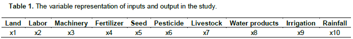
Land: This is defined as the total utilized agricultural land, that is cultivated land. This included land sowed (crops and vegetables), those under fallow, land occupied by ornamental plants and fruits, as well as those used as permanent meadows and pastures (TUIK). This is measured in thousand hectares (1000 Ha). Data on this was gotten from TUIK with the exception of the year 2000. This was complemented by the WDI which had the Figure for 2000. It is represented as ‘x1’
Labor: Agricultural labor consists of economically active labor force of a country that is engaged in agricultural activities for living. This includes crop production, animal husbandry, hunting, forestry and fishing. The data considered 15 years of age and above as the active working population. The source of this data has been a little challenging. Turkey until 2005 was recording their labor force statistics based on the ordinary household labor force survey, but adopted the more harmonized European Union Labor Force Survey (EU LFS) from 2005. With the study period under review, this would mean that our data span the period between these two different surveys. This means that using any of them will mean the unavailability of data for a significant amount of years, which can be extrapolated. We settled for the EU LFS for two important reasons; its harmonized nature and the fact that we have to extrapolate for 5 years backwards instead of 10 years ahead if we had chosen the other one. The data was gotten from TUIK.
Agricultural machinery: A lot of items come under this category. However, monetizing these items would have been good but it is almost impossible especially for a national aggregated data like this. Unlike livestock units (LSU) for livestock and labor force survey (LFS) for labor, there is no known aggregation technique to include all type of machinery even though there is data on their respective quantities. Because of the aforementioned problem the data on machinery is limited to the two most important and highly used machines; tractors and combine-harvester. Their combined number is used.
Fertilizer: This data was extracted from the database of the International Fertilizer Association (IFA) of which Turkey is a member. The most highly used plant nutrients are considered; Nitrogen (N), Potassium (K2O) and Phosphorous (P2O5). The summation of the weight of each of the nutrients is represented in the study in thousand tones nutrients. However available data fell short of two years, which was then extrapolated, that is the data did not include the years 2013 and 2014.
Seed: Considering the importance of seeds as a direct input to agricultural crop production, the study considered in tones, the combined weight of all seeds in the production of all crops and plants in Turkey. These include cereals, legumes, tubers and ornamental plants. The whole data with the exception of 2014 (extrapolated) was gotten from FAOSTAT.
Pesticide: Pesticide use by so far is the variable with most missing data which had to be extrapolated. Even though there are different type of chemical used in agriculture, they are basically grouped into five; insecticides, herbicides, fungicides/bactericides, rodenticides and acaricides. However, an allowance was made for other chemicals that are used but has no classification under these five. Data for this is found both in FAOSTAT and TUIK, but that of FAOSTAT has a lot of inconsistencies even though it covers the entire period of study. That of TUIK covers from 2006 to 2013. We used the information from TUIK but had to extrapolate for the missing data. They are measured in tones.
Livestock: The agricultural output from livestock is directly linked to the number of animals available. They are the main source of protein, especially from their meats and eggs. However, livestock comes in different shapes, breeds and sizes. Even geographically, there is vast difference between the same kind of livestock. This makes aggregation difficult. Livestock units (LU) are an aggregation procedure used to find the total number of livestock from different categories of livestock. This technique however, varies from region to region. The designated regions are North Africa, Sub-Saharan Africa, South Africa, North America, Central America, South America, Asia, Eastern Europe, Oceania Developing, USSR and OECD. The geographical classification of Turkey as a country has been a controversy. It can be classified as Near East country, Eastern Europe and an OECD member. This poses a problem on which unit to use. We consequently settled for the OECD criterion which is less geographically defined. Regions and countries that are in the tropics use the famous Tropical Livestock Unit (TLU). In order to standardize the data, we considered Global/International Livestock Unit (ILU). In this technique, all regions are compared to that of North America, with cow as the reference (referenced as 1). The livestock considered are cattle, buffalo, sheep, goats, pigs, horses, mules, camels, asses, chickens, ducks, turkeys, geese and rabbits.
There are two major limitations to this aggregation with regards to our data. Firstly, Turkey does not have official records on the number of rabbits, but FAO has a fixed estimation of 50000. Secondly Beehives are livestock, however there is no known LSU for their measurement; hence information about it is omitted from our measurement.
n = number of species/type, ILUi= ILU for species/type
Water products: This input complement livestock in the provision of agricultural output especially protein related products. This input is normally not considered in most studies, however it is very important to the agricultural output of some countries. We believe Turkey, which has almost half its border as coastline in addition to the numerous inland water systems, owes a significant amount of its agricultural output to its waters. The data comprises the total amount in tons of sea products, aquaculture and freshwater products. Data for 2001, 20013 and 20014 were extrapolated.


Irrigation: This input is captured as the number of dams constructed for irrigation purposes. Normally in efficiency and productivity analysis studies, this is captured as the proportion of arable land that is irrigated. However, we felt that in order to capture irrigation as an input to agricultural output, it should be the number of irrigation facilities used. If irrigated land is considered, there will be confliction with the total agricultural land which in itself is an input. These records were gotten from DSI database.
Rainfall: Rainfall is an important input in determining the aggregate agricultural output of any country. It is such an important input that its quantity, pattern and timing can have a disastrous effect on agricultural output as a whole. Even irrigation-dependent production needs rainwater to reinforce the dams for efficient operation. This data records the annual rainfall in millimeters (mm), all from DSI database.
The variable representation of inputs and output in the study is shown in Table 1.
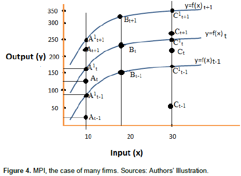
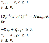
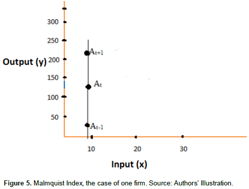
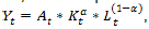
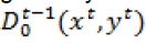 means the productivity of that firm at the current year ‘t’ compared with the previous year’s ‘t-1’ frontier or technology. That is the one in the brackets is the firm in question and what is outside the bracket is the reference technology.
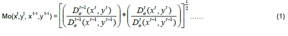


.png)


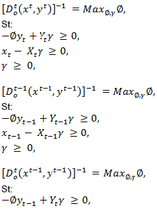
 the distance function will be the ratio of the point of interest to the corresponding point on the frontier. Example for a point in year ‘t’ will be
 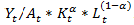 Substituting the various distance function into equation 1, that is the original Malmquist index formulation;