The paper examines the status and determinants of poverty and inequality among rural households in Girar Jarso district of Central Ethiopia. To measure the status of poverty and inequality, the study made use of cost of basic need approach, Foster-Greer-Thorbecke indices and Gini coefficient. Based on the survey of 120 households, the logistic model was estimated. A three-stage sampling procedure was applied for selection of respondents. The poverty line is found to be 4315.7 Ethiopian Birr. The incidence of poverty was computed to be 45% with an average poverty gap and squared poverty gap of 18.6 and 9.99%, respectively. The Gini coefficient was calculated to be 0.33. The logit model shed light on the demographic and socioeconomic characteristics of households behind the persistence of poverty. The result revealed that poverty is strongly linked to family size, remittance, farm and non-farm income and receiving food aid. The findings suggest also that livelihood diversification, encouraging flow of remittances, promotion of non-farm activities, besides agricultural intensification, and appropriate target to avoid distortionary effects of food aid will constitute an important strategy to accelerate poverty reduction.
Achieving sustainable economic growth with a particular focus on eradicating extreme poverty and hunger has become the key development goal for governments around the world, as reflected in the Sustainable Development Goals (World Bank, 2017). The World Bank (2014) also set an ambitious goal of reducing, to no more than 3%, the fraction of the world's population under the canopy of poverty by 2030. However, there are around 1.2 billion people in extreme poverty in the world (World Bank, 2015). Globally, substantial progress has been made in reducing poverty in the past few decades. The share of African population in absolute poverty declined from 56% in 1990 to 43% in 2012 (Beegle, 2016). Although Ethiopia has long been known as the cradle of humanity, poverty remains dauntingly widespread and pervasive. By any standard, the majority of people in Ethiopia are among the poorest in the world. Ethiopia has achieved a remarkable economic growth on average of 10.6%, in comparison with an average population growth rate of 2.6%; this implies that the average annual per capita income growth rate was 8.4%.
However, because of high population growth, the absolute number of the poor has remained unchanged at some 25 million over the past 15 years. Poverty head count has fallen from 45.5% in 1995 to 26.0% in 2012/2013. It is slightly higher in rural areas (30.4%) than in urban areas (25.7%). Many rural Ethiopians cycle around the poverty line, moving in and out of poverty during the course of a year. Income of the rural poor is 7.8% on average; far from the poverty line, while it is 8.0% for the urban poor. The poverty gap was also reduced but not the severity of poverty. The country is registered to be the poorest in Sub-Saharan Africa with a Human Development Index of 0.448 and Multidimensional Poverty Index of 0.564, which gives a rank of 174 out of 188 and second from the last (Niger) (MoFED, 2012; UNDP, 2015; OPHI, 2016). Ethiopia, as in other countries in the Horn of Africa, is now associated with famine and it has become the iconic poor country (Maxwell, 2007).
Over the last several decades, there has been extensive works on analysis of poverty in Ethiopia. The research interest was strengthened with the decision of many countries to adopt the UN Millennium Declaration exerting as much effort as possible to achieve the MDGs. Many researches revealed that poverty experienced in the last several decades results from a number of structural factors; prolonged conflict, adverse geographical condition, vulnerability to shocks, decline in land holding, irregular supply of inputs, poor access to education, fragile food security, limited access to healthcare and lack of infrastructure, weak institutional structures, rapid population growth, failures in credit, land and extreme environmental degradation (Porter, 2015; Jakiel, 2016; Gecho, 2016). An over-reliance on agriculture, poor asset ownership, poor education, and trivial levels of livelihood diversification are all to blame. Besides, the country suffers spells of drought, with resulting famines and such conditions have a strong influence on the living standards of the whole population (World Bank, 2015).
Ending poverty in all its forms everywhere has been an important component of the SDGs setting out goals and targets to be met by the year 2030 (UNDP, 2015). The adoption of a global goal only makes sense if progress can be monitored. Poverty analysis is a natural point of departure. For a country analysis to meet the SDGs, designing a strategy, analyzing the magnitude and investigating the root causes of poverty has a paramount importance. Since poverty reduction is not an instantaneous process, continuous and systematic analysis is very crucial (MoFED, 2012; World Bank, 2017). A number of studies have been done at micro level to examine the extent and determinants of poverty in rural Ethiopia (Bogale et al., 2005; Dawit et al., 2011; Abebe, 2017; Bogale, 2011; MoFED, 2012; Sharma, 2014). Most of these studies are aimed at assessing the extent of poverty and explain relative changes which occur in the incidence of poverty due to policy changes.
The empirical results of these studies reflect the severe poverty level that continues to prevail in rural Ethiopia and poverty has multiple causes that exhibit economic, social and political characteristics. However, what have so far been studied in Ethiopia, much if not all, concentrate on and reflect the national picture. But studies and analysis at an aggregate level do not necessarily reflect the situation at grass root level. Dercon and Krishnan (1998) strongly advised that one should be careful about the implications derived from measurement and factors of poverty at the national level, because it hides many important differences that exist in different locations. The road coming out of poverty is rarely a smooth one. The dream of ending global poverty by 2030 is a highly aspirational objective, but is not entirely beyond reach with concerted efforts and commitment from individual countries as well as the international development community (World Bank, 2015). In order to combat such incapacitating problem and its exit time considering very scarce resources available to be allocated for the purpose, the poor must be properly identified and an index taking the intensity of poverty suffered by the poor into account needs to be constructed (Bogale, 2011).
Poverty everywhere is a rural phenomenon and it is caused by dynamic factors that need persistent exploration in order to know its causes at a particular time. Most Ethiopians are rural dwellers and subsistence farmers, and the poorest 40% tend to be even more likely to live in rural areas and engage in agriculture (World Bank, 2016). So far analytical works that scrutinize poverty conducted in Girar Jarso is at best scanty. Most researches focus on the determinants of poverty at an aggregate level. Measurement and analysis of poverty at a disaggregated level is a necessary condition to make the poor an agenda by policy makers on that particular area. The outcomes of the analysis should give a clear picture on the situation in order for decision-makers to be able to identify critical areas for intervention (MoFED, 2012; SESRIC, 2015). To eradicate poverty, successive regimes have launched several poverty alleviation programmes to curtail problems of poverty in the country. These programmes have ensured reduction in poverty. However, the pace of poverty reduction over the past decade has been slow. This phenomenon calls for assessment of poverty and as such, the objective of this study is to assess the status of poverty, measure income inequality and identify the major determinants of poverty.
Study area
Girar Jarso is located in Central Ethiopia 112 km away from Addis Ababa on the way to Bahirdar, with an area of 401.9 km2. The central highlands have long been considered Ethiopia’s most famine-prone areas (Maxwell, 2007). According to Zone Finance and Economic office report of 2004 E.C, the population of the woreda is closed to 76,921 (Male 39,387 and Female 37,534). The average annual temperature ranges from 15 to 18°C, while the average annual rainfall varies between 1200 and 1400 mm. The land holding size on average is estimated to be 3.2 ha. The district is divided into 17 peasant associations with a total of 12,062 farm households (DARDO, 2009) (Figure 1). Mixed farming is the mainstay of the household economy, intensively carried out by those who have land and livestock.


The farming system is rain fed and is characterized by low productivity, low use of farm inputs, traditional farm practices, poor soil fertility, water logging and other related problems. The landless are engaged in sharecropping and other off farm income generating activities like daily laborer. Agricultural products are consumed at home and partly sold to earn cash to meet other household needs, educate children, and contribute to social affairs. The main crops grown include cereals (barley, wheat and teff), pulses (horse bean, chickpea, and lentil), fruits and vegetables (apple, cabbage, kale, onion). Livestock contributes to the subsistence requirement of the population particularly from small ruminants. The major livestock species kept by farmers in the area includes shoats, cattle, donkey, mule and horse. Like elsewhere in the country, the production and productivity of this sub sector is very low.
Sampling procedure
The analysis of poverty in this paper is based on a household survey conducted in Girar Jarso district in Central Ethiopia. The rural household was taken as a basic unit of analysis. The research design followed a multi stage sampling method (systematic and random) at woreda, village and household levels, respectively for selection of desired sample respondents to generate the required primary data. In the first stage, Girar Jarso district was selected purposively from 14 Woredas of the zone based on frequency of shocks like drought or being in famine prone area, food relief program and the subsequent death of cattle during drought season within the central Showa highlands as criteria. In the second stage, four peasant associations, namely, Torbanashe, Addisge, Dire Doyyo and Koticho were selected randomly from a list of peasant associations in the district. In the third stage, sample households were randomly drawn from a complete list of respective peasant association members in conformity with the proportionate to size random sampling procedure. In total, the survey covered 120 households.
Data were collected using both primary and secondary sources. Before conducting the field survey, three enumerators with practical knowledge of the area and well conversant with the culture and language were recruited. The enumerators were diploma holders. However, a detailed discussion was held with them about the interview schedule and they were trained on understanding the questions, interpretation and translation of concepts which improved their confidence and to make amendment in the interview schedule accordingly. To obtain information on poverty, empirical data were collected through structured questionnaires. Discussions with key informants were also held. The enumerators collected the required data under a close supervision of the researcher. The structured questionnaires on demographic, economic and institutional aspects were posed to heads of households. The filled-in interview schedules were thoroughly checked every day on the spot for completeness and for re-interview if problem occurred. Beside the primary data, relevant documents to the study, books, previous working literatures, statistics, and checklists of facts and figures were collected from different government offices of the Woreda. Unpublished materials were also used.
Method of data analysis
After the data collection and retrieval, the data were first sorted out, edited, coded and analyzed using Excel and Statistical Package for Social Sciences (SPSS version 16.0). The research then used descriptive statistics like percentages, means and standard deviations, and inferential statistics like Chi-squares and t-test. The Costs of Basic Needs (CBN) approach, Foster-Greer-Thorbecke (FGT) indices, Gini coefficient, Watts index and econometric model were also employed to address the stated objectives of the study.
Setting poverty line
The first step in measuring poverty is defining an indicator of welfare such as income or consumption per capita (Khandker, 2009). Consumption expenditure or income has been traditionally used as measure of household poverty. But consumption is typically preferred to income as it better captures long run welfare. It is considered as an adequate measure of household welfare in developing countries as it is better able to capture household’s consumption capabilities. Consumption may also better reflect household ability to meet their basic needs. Income is one of the factors that enable consumption, though consumption also reflects a household access to credit and saving at times when their income was too low. Hence consumption is a better measure of household welfare than income (World Bank, 2016). The analysis here is based on the consumption expenditure dataset of the sample households.
There are several approaches to construct the poverty lines. The most popular method of poverty measurement have used the nutritional norm and defined poverty in terms of minimum calorie requirements. The Cost of Basic Needs (CBN) is one of these different approaches, where the total poverty line is constructed as the sum of a food and a non-food poverty line (Greer, 1986; Khandker, 2009). According to Ravallion (2016), three steps in the process of defining absolute poverty lines were used. This includes choosing a welfare indicator, establishing a poverty line and aggregating poverty data. The first step involves specifying a reference level of utility representing a minimum standard of living. The research employs a consumption bundle (2300 Kilo calorie/adult equivalent/day) considered adequate for an adult to lead an average physical life under normal conditions based on estimation of the Ethiopian Nutrition and Health Research Institute (EHNRI, 1997).
Next, consumption expenditure as a money metric threshold between the poor and non-poor associated with the reference utility level was identified. In this case, households were divided into quartiles according to their consumption expenditure per adult equivalent. The choice of reference group was determined on the basis of the commitment the governments want to make in terms of allocating resources to poverty reduction programs. It was reasonable to choose the population belonging to the bottom quartile as a reference group (Kakwani, 2010). The food poverty line is obtained by selecting baskets of food items which are reasonably consumed in a given setting and then calculating which basket yields the specific calorie minimum at the lowest cost under the prevailing prices. The cost of this basket defines the food poverty line.
The food consumption behavior of the reference group accesses to determine average quantities in per adult equivalent of basic food items that makeup the reference food basket. In this case, the basket is made up of the mean consumption levels (purchase, remittance, from aid, and own production) of 13 food items. The calorie value of each food items is established from the food nutrition table of Ethiopian Health and Nutrition Research Institute. The total calorie from consumption of this basket of average quantity per adult by an individual is:
∑Qi Kcal = T *, with T ≅ T *. But T *' ≠ T
where T* is the total calorie by individual adult from consuming the average quantities, Qi is the average quantity per adult of food item ‘i ‘consumes by individuals, Kcal is the caloric value of the respective food item ‘i‘ consumed by individual adult and T is the recommended calorie of per day per adult.
The average quantity per adult of each food item scales up and down by a constant value so as to provide total of 2300 Kilo calorie/adult equivalent/day before doing any activities. Then, multiply each food after scaling up by the median price and sum up to get a food poverty line. The method of deriving the non-food poverty line is done by choosing some non-food considered essential. However, since there is no absolute standard for minimum non-food requirements similar to that of food that has a standard calorie intake as a basis, constructing the non-food poverty line remains arbitrary (SESRIC, 2015). The non-food needs were obtained by examining the non-food expenditures per adult equivalent per year for households in the lowest income quartile.
Poverty indices
Among the various methods of quantifying poverty, the Foster, Greer and Thorbecke (FGT) formula (Foster, 1984) is the most widely used method. With the help of these indices, the head count, poverty gaps and squared poverty gaps were calculated. The formula has been successful in providing a quantitative description of the spread, depth and severity of poverty in populations. These classes of poverty indices were followed to scrutinize the extent of poverty at the household level. The mathematical expression of the model is specified as:
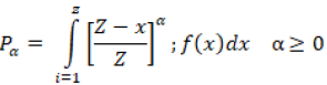
where Pα is the poverty measure, Z is the poverty line, x is the income of households, N is the sample population, q is the number of poor, and α is the poverty aversion parameter or the weight attached to severity of the poor. The measures are defined for α³0. For α = 0, P0 = f (z), the cumulative income distribution at the poverty line Z. In other words, for α = 0, all poor are given equal weight and P0 equals the head count ratio. If α = 0, Pα, P0 becomes:
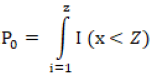
where I (.) is an indicator function that takes on a value of 1 if the bracketed expression is true and 0 otherwise. So if expenditure x is less than the poverty line (Z), then I (.) equal 1 and the household would be counted as poor. Head count index reflects the proportion of the poor in total population. It literally counts heads, allowing policymakers and researchers to track the most immediate dimension of the human scale of poverty (Morduch, 2005; SESRIC, 2015). The greatest virtues of the headcount index are that it is simple to construct and easy to understand. However, it does not take the intensity of poverty into account, it violates the transfer principle and it does not indicate how poor the poor are, and hence does not change if people below the poverty line become (Khandker, 2009; Ravallion, 2016).
A moderately popular measure of poverty is the poverty gap index, which adds up the extent to which individuals on average fall below the poverty line, and expresses it as a percentage of the poverty line. More specifically, define the poverty gap (G
i) as the poverty line (Z) less actual income (x) for poor individuals; the gap is considered to be zero for everyone else. Using the index function, we have G
i =
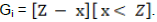
.
The index can be normalized by being expressed as percentage shortfall of the average income of the poor from the poverty line (Sen, 1979). If

then the poverty gap index (P
1) may be written as:
The poverty gap is intrinsically meaningful, taking us from counting people to counting shortfalls of income or consumption. It captures the mean aggregate income shortfall relative to the poverty line. However, the income gap ratio is not a good measure of poverty as P1 is sensitive to the depth of poverty but not to its severity. It is the minimum cost of eliminating poverty, because it shows how much would have to be transferred to the poor to bring their incomes or expenditures up to the poverty line (as a proportion of the poverty line). This measure is an indicator of the potential savings to the poverty alleviation budget from targeting; the smaller the poverty gap index, the greater the potential economies for a poverty alleviation budget from identifying the characteristics of the poor. The poverty gap index violates Dalton’s transfer principle (Khandker, 2009; SESRIC, 2015; Ravallion, 2016)
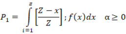
To construct a measure of poverty that takes into account inequality among the poor, many researchers use the squared poverty gap index. This is simply a weighted sum of poverty gaps (as a proportion of the poverty line), where the weights are the proportionate poverty gaps. This measures the mean of the individual poverty gaps raised to a power reflecting society’s valuation of different degrees of poverty. Hence, by squaring the poverty gap index, the measure implicitly puts more weight on observations that fell well below the poverty line (SESRIC, 2015; Ravallion, 2016). The measure lacks intuitive appeal, and because it is not easy to interpret it is not used widely (Khandker, 2009). Formally,
This depicts severity of poverty by assigning each individual a weight equal to distances from the poverty line. Hence, P2 takes into account not only the distance separating the poor from the poverty line, but also the inequality among the poor.
Measure of inequality
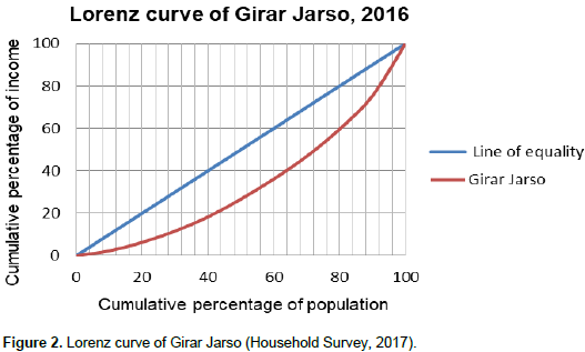
Income inequality is measure by most widely used technique known as Gini coefficient. In other words, it is the ratio of the area between the Lorenz curve and the diagonal equality line to the total area of the triangle. The Lorenz curve graphically illustrates the relationship between population shares and income shares. The closer the Lorenz curve is to the diagonal, the more equal is the distribution. The Gini coefficient varies between a value of 0 that corresponds to perfect income equality (that is, everyone has the same income) and 1 corresponds to perfect income inequality (that is, one person has all the income, while everyone else has zero income). Gini coefficient satisfies Pigou-Dalton transfer sensitivity, symmetry, mean independence and population size independence criterion (Khandker, 2009; SESRIC, 2015; Ravallion, 2016).
Mathematically,

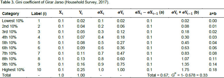
where GP is Gini coefficient, sXi is cumulative value for the population up to category i, sYi is cumulative value for the income up to category i and i is label (for the population or income). Sen (1976) has proposed an index that sought to combine the effects of the number of poor, the depth of their poverty, and the distribution of poverty within the group. The index is given by
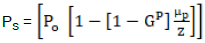
where P0 is the headcount index, µP is the mean income (or expenditure) of the poor, and GP is the Gini coefficient of inequality among the poor. The Sen Index can also be written as the average of the headcount and poverty gap measures, weighted by the Gini coefficient of the poor, giving:
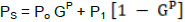
where PS is the Sen’s poverty index, Po is the head count index, P1 is the poverty gap index and GP is the Gini coefficient. In value of PS ranges from 0 (no one is below poverty line) to 1 (no one has any income).
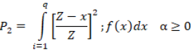
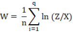
The Watts index according to Ravallion (2016) is a good poverty measure to penalize inequality among the poor and is perhaps the best. It satisï¬es all the desirable axioms or a poverty measure and is increasingly used in generating the poverty incidence curve. Under the focus axiom, the measure should not vary if the income of the non-poor varies; under the monotonicity axiom, any income gain for the poor should reduce poverty; and under the transfer axiom, inequality-reducing transfers among the poor should reduce poverty (Khandker, 2009). The Watts proportionate poverty gap of person i can deï¬ned as ln (Z/X) if the person is poor (X< Z); otherwise, then the gap is zero, of course. Note that this is not the same as the proportionate poverty gap (1– X/Z), which is why we shall call ln (Z/X) the Watts proportionate poverty gap. Now take the mean of these proportionate poverty gaps in the population. If incomes are ordered such that X≤ Z if and only if i < q, q is the number of poor households, then the Watts index is:
Descriptive statistics
The descriptive statistical tools like mean and standard deviation were employed for analysis and interpretation of household quantitative characteristics. Besides, inferential statistics such as t-test and Chi-square tests were used for interpretation of data and drawing conclusions.
Specification of the model
To identify the major determinants of poverty, a binary logit model was applied. The dependent variable is binary whereby the sample household were categorized into poor (y = 1) and non-poor (y = 0) on the basis of consumption expenditure. Logistic regression model is commonly recommended as an appropriate probability model in such a situation. The model is mathematically specified as:
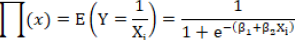
where e is the base of the natural logarithm which is approximately equal to 2.718, Xi is the ith explanatory variable, Õ (x) is the probability that an individual will make a certain choice, where Xi and α and b are regression parameters to be estimated. The probability that a household belongs to the non-poor will be (1-Õ (x)).
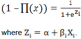
Therefore, to get linearity both in variable and in parameters the natural log of the odd ratio should be taken. As p goes from 0 to 1, the logit goes from –α to α, that is, although the probabilities lie between 0 and 1, the logit Z are not so bounded (Gujarati, 1988). The model can be estimated through iterative maximum likelihood procedure. The coefficient of the logit model represents the change in the log of the odds associated with a unit change in explanatory variable.
where Zi is the poverty status of households; X1, X2………….. Xn are the explanatory variables; β0 is intercepted terms; β1, β2…….. βn are the partial regression coefficients of parameters; I is the ith observation; and Ui is the stochastic disturbance or the error term. If the disturbance term is taken in to account, the logit model becomes:
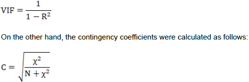
Multicollinearity has been checked before running the model using variance inflation factor (VIF) and contingency coefficients (C). VIF shows how the variance of an estimator is inflated by the presence of multicollinearity (Gujarati, 2004). Each selected continuous variable is regressed on the other, so that the coefficient of determination (R2) would be constructed. A variable is said to be highly collinear, if R2 exceeds 0.9 or VIF exceeds 10 (Gujarati, 1995). VIF is expressed as:
where C is the contingency coefficient,
 2
2 is Chi-square and N is the total sample size. The values of C range between 0 and 1, zero indicating no association between the variables and values close to 1 indicating a high degree of association, which means high degree of multicollinearity.
Hypothesis
Dependent variable
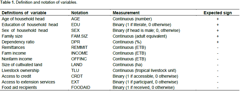
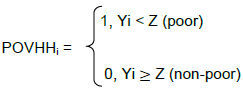
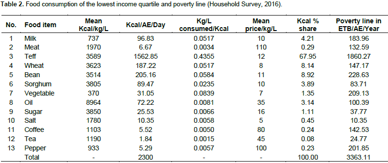
The dependent variable for this study is household poverty, which is dichotomous. The information to categorize households into two groups was obtained by comparing the total consumption expenditure per adult equivalent per annum to the poverty line. This poverty line was computed based on the amount of calorie requirement (2300 Kcal/adult equivalent/day) plus average expenses needed for non-food items of the lowest income quartile (Table 1).
where POVHHi = household food security status of the ith household, Yi = Consumption expenditure of households, Z = Poverty line. It is hypothesized to be a function of the following explanatory variables, selected on the basis of review of literature, past research findings, experts and authors’ knowledge of the poverty situation in the area.


where C is the contingency coefficient,
2 is Chi-square and N is the total sample size. The values of C range between 0 and 1, zero indicating no association between the variables and values close to 1 indicating a high degree of association, which means high degree of multicollinearity.
Hypothesis
Dependent variable
The dependent variable for this study is household poverty, which is dichotomous. The information to categorize households into two groups was obtained by comparing the total consumption expenditure per adult equivalent per annum to the poverty line. This poverty line was computed based on the amount of calorie requirement (2300 Kcal/adult equivalent/day) plus average expenses needed for non-food items of the lowest income quartile (Table 1).
where POVHHi = household food security status of the ith household, Yi = Consumption expenditure of households, Z = Poverty line. It is hypothesized to be a function of the following explanatory variables, selected on the basis of review of literature, past research findings, experts and authors’ knowledge of the poverty situation in the area.
Age of household head
It is a continuous variable measured by number of years. As age of household head increases, there is greater tendency to acquire knowledge and experience (Shete, 2010; Dawit et al., 2011; Sharma, 2014). Thus, it is hypothesized that age and poverty are negatively correlated.
Sex of household head
Household head is a person who economically supports or manages a household or for reason of age is considered as head by other members of the household. It is a dummy variable taking a value of 1 if male and 0 otherwise. Households headed by male have more access to agricultural technologies and more security to farmland than female headed ones (Bogale et al., 2005; Shete, 2010; Sharma, 2014). It was hypothesized that male headed households are less likely to be poor than female headed ones.
Education
It is believed to be a necessary condition to equip individuals with the knowledge of how to make a living. Education is a necessary factor for stimulating a country’s economic growth as it allows people to be more productive and provides more opportunities for its citizens (Sharma, 2014; Muhammedhussen, 2015; Jakiel, 2016). Literates are eager to get information and use it. Hence, it is supposed that households who have had at least primary education or informal education are the ones to be more likely to benefit from agricultural technologies and thus become non poor.
Family size
It represents the total family size adjusted to adult equivalent. As family size increases, obviously the probability of having economically non active members or children and doddering ages is higher. As family size increases, household resource per head decreases (Dawit et al., 2011; Sharma, 2014; Muhammedhussen, 2015). Hence, it is hypothesized that family size and poverty are positively related.
Dependency ratio
As a continuous variable, it is the ratio between economically inactive (age less than 15 and above 65) with active labor force (age between 15 and 65) with in a household. When a large family size corresponds with the availability of adequate adult labor, it can have a positive effect. A household with high economically non active members shows high dependency ratio and it is more likely to be poor (Bogale et al., 2005; Shete, 2010; Bogale, 2011; Sharma, 2014; Muhammedhussen, 2015). Therefore, it is hypothesized that dependency ratio and poverty are positively associated.
Remittances
Remittances from other sources of finances are an important continuous explanatory variable that can be gauged as one of the indicators of measuring poverty. The values of remittance received are critically important in supporting inclusive growth and reducing poverty through boosting household consumption (UNDP, 2015; Berisso, 2016). Remittance is done as part of their indigenous culture of helping each other. It is expected that having relative economic support from abroad and urban areas within the country has positive impact in reducing the poverty status of households.
Farm income
It is a continuous variable explaining the characteristics of poor and non-poor households. The higher the level of income from farming, the lesser would be the likelihood of household to become poor. Therefore, farm income was hypothesized to be negatively related with household poverty.
Non-farm income
Agricultural production may not be the sole source of income for the rural household. Income earned from non-farm activities is an important continuous explanatory variable that determines household poverty. The success of households in escaping from poverty depends on their ability to get access to non-farm job opportunities. Hence, it was hypothesized that households engaged in non-farm activities are better endowed with additional income and less likely to be poor (Bogale, 2011; Dawit et al., 2011; Babu and Afera, 2013).
Livestock ownership
As a continuous explanatory variable, it represents the livestock number in Tropical Livestock Unit owned per adult equivalent. It is an important variable because households generate some proportion of their income and food items from livestock. The larger the number of Tropical Livestock Unit, the better the level of production and income (Bogale et al., 2005; Dawit et al., 2011; Bogale, 2011; Muhammedhussen, 2015). Therefore, it was hypothesized that households having more number of livestock have less probability to be poor. The livestock ownership is negatively correlated with poverty.
Cultivated land size
It is a continuous variable representing the total landholding of the household measured in hectares. Total cultivated land owned by household is important resource for food production and is negatively associated with poverty status (Bogale et al., 2005; Shete, 2010; Muhammedhussen, 2015). Thus, it is expected that size of cultivated land will have positive impact on reducing poverty.
Access to credit services
Access to credit is a dummy variable with a value 1 if the households received credit, either from formal or informal sources and 0, otherwise. Those households who received the credit wanted to have better possibility to spend on activities they want. They can improve production and productivity by adopting different agricultural technologies. Credit access eases access and use of all production inputs; improved seeds or breed, chemical fertilizer, agrochemicals, feed supplement or livestock medicine (Dawit et al., 2011). It was hypothesized that access to credit affects positively on reducing household poverty.
Access to extension services
It is a dummy variable taking a value of 1 if household has access to extension service and 0 otherwise. The provision of extension services to the farming households directly affects their knowledge, productivity and income; mainly because they have a tendency of using production technologies and learn to practice modern production techniques and are prone to change (Dawit et al., 2011). It was expected to influence household poverty status negatively.
Food aid receiving
It is a dummy variable taking the value 1, if the household receives food aid 0 otherwise. Despite the huge amount of aid received through Productive Safety Net Program, its impact as development resource is inconclusive in both theoretical and empirical evidences (Calfa, 2010). Food aid can increase resources for current consumption; increase and improve the nutritional status of the poor. Thus, by directly alleviating hunger and poverty, food aid is hypothesized to serves as a wage for the poor.
Poverty status
The food poverty line which is calculated from the data available is found to be 3363.11 Ethiopian Birr/adult equivalent/annum (Table 2). The non-food needs were obtained by examining the average non-food expenditures/adult equivalent/year of households in lowest income quartile households. The mean value was 952.6 Ethiopian Birr/adult equivalent/annum. Adding this to the food poverty line gives a total poverty line of 4163.11 Ethiopian Birr/adult equivalent/annum. Compared to other studies at disaggregated level, the poverty line in terms of Ethiopian Birr/adult equivalent/annum of Girar Jarso was found to exceed what Bogale et al. (2005) ranging from 460 to 715 computed for districts of Alemaya, Hitosa and Merhabete in 2005, Babu and Afera (2094) for Gulomekeda, Abebe (2976) for Chencha and Abaya in 2017, Shete (758.27) in 2010, Bogale (1468) for Hararghe highlands in 2011 and still greater than the national average set at 3781 Ethiopian Birr/adult equivalent/annum in 2011 prices (MoFED, 2012).
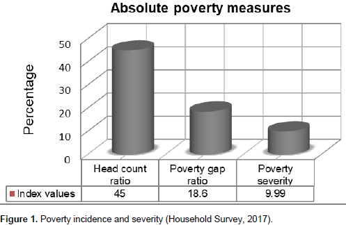
This poverty line is used to estimate the poverty indices in the study area. Accordingly, the poverty indices calculated using the Foster-Greer-Thorbecke measures were found out to be 0.45, 0.186 and 0.099 for head count, poverty gap and poverty severity, respectively (Figure 2). The resulting poverty estimates show that the percentage of poor people is about 45%, which is more than the regional and national averages (29.3 and 29.6% respectively), Chencha and Abaya (29.8%) (Abebe, 2017), Alemaya and Hitosa (35 and 24%, respectively) (Bogale et al., 2005), and Hararghe highland (35.6%) (Bogale, 2011), but lower than Zeghe peninsula (68.5%) (Shete, 2010) and Gulomekeda (51%) (Babu and Afera, 2013). This indicated that this proportion of households in Girar Jarso woreda live under the canopy of poverty; that is, this share of the population cannot afford to buy a basic basket of goods enabling to get the minimum calorie required (2300 kilo calorie per adult equivalent per day) adjusted for the requirement of non-food items expenditure.
The poverty gap index of 0.186 implies that mean per capita income shortfall of the poor relative to the poverty line was 801.69 Ethiopian Birr/adult equivalent/year. With 3.98 adult equivalents average family size in the area, there was an income shortfall of about 3190.73 Ethiopian Birr per year for a household. Since the district has a total number of 12,062 farm households, it would be 38,486,539.4 Ethiopian Birr per year overall shortfall. It is, therefore, a much more powerful measure than the head count ratio because it takes into account the distribution of the poor below the poverty line and also reflects the per capita cost of eliminating poverty. The poverty gap is less than half of the headcount ratio. In effect, many people are concentrated around the poverty line.
The per capita cost of eliminating poverty in the study area was higher than Alemaya, Hitosa and Merhabete computed in 2005 by Bogale et al. (2005) (3.5, 3.52 and 13.5%, respectively), Hararghe highland (9.1%) calculated by Bogale (2011) and still higher than the 7.8% of the poverty line of the national average (MoFED, 2012). But, it is lower than Gulomekeda (15%) computed by Babu and Afera (2013). Similarly, squared poverty gap in consumption expenditure of 9.99% implies that there is a high degree of inequality among the lowest quartile population. Thus, for 9.99% of the total 120 households, more weight has to be given as they are the poorest of the poor. This result confirms the existence of greater proportion of poorest of the poor households in Girar Jarso than Alemaya, Hitosa and Merhabete (0.74, 0.98 and 3.4%, respectively), Gulomekeda (5.9%), Hararghe highland (3.6%) and national average of 3.1%. But, it was equivalent to what Shete has computed as the poorest of the poor in the Peninsula (18.7%).
Income inequality
The Gini coefficient for countries with highly unequal income distribution typically lies from 0.5 to 0.7 and for countries with relatively equitable income distribution, it is in the order of 0.2 to 0.35 (Todaro and Smith, 2009). Gini coefficient of Girar Jarso is found to be 0.33, more than the national average. It is also not much far from zero, shows existence of equality (Table 3). With a Gini coefficient of 0.30, Ethiopia remains the most egalitarian countries in the world (World Bank, 2016). Generally, Girar Jarso has relatively low inequality in per capita income. It is relatively higher as compared to the Gini coefficient of a study which was done in Hararghe highlands (0.29) (Bogale, 2011).
Although inequality remained low, the very poorest might became poorer, posing a challenge to the goal of shared prosperity in Ethiopia. The same source revealed that there was a lower growth rates in consumption observed among the bottom 40%. The highest growth rates were experienced by the fourth decile, but the poorest 10% experienced a decline in consumption. As a result, reductions in poverty rates were not matched by reductions in the depth and severity of poverty. Moreover, when the result is compared to that of Torado’s categorization, the income distribution is comparatively equal because the 0.33 is in the rage of equitable distribution. But, it implies the majority of them are equally poor. Sen’s poverty value was found to be 0.165.The Lorenz curve plots the cumulative share of income earned on the y-axis by households ranked from the bottom to the top on the x-axis. In a region with perfect equality, the Lorenz curve would be a perfectly straight 45° line. This Gini ratio gets smaller as the Lorenz moves closer to the diagonal and attains a value of zero when absolute equality is achieved. The Watts index, computed by dividing the poverty line with income, taking logs, and finding the average over the poor is found to be 14.64 (Figure 2).
Descriptive statistics
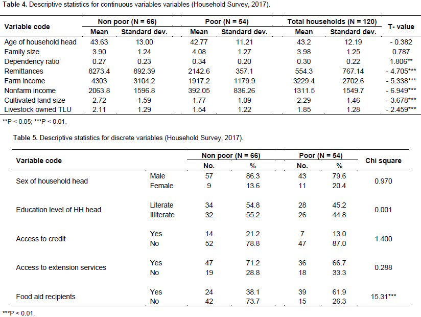
The descriptive statistics for continuous and discrete variables were presented separately. The continuous variables which are helpful to observe differences among the poor and non-poor households include age of household head, family sizes, dependency ratio remittances, farm income, non-farm income, cultivated land size and number of livestock owned. Family sizes and dependency ratio of the poor were higher than non-poor households. Age of household head, remittances, farm income, non-farm income, cultivated land size and number of livestock owned on the other hand were higher among non-poor households than the poor. Though the family sizes in adult equivalent and dependency ratio of the poor were higher than the non-poor households, this difference was only statistically significant at the 5% significance level for dependency ratio.
On the other hand, remittances, total farm income, total off farm income, cultivated land size and number of livestock owned were higher and statistically significant at the 1% significance level among non- poor households compared with the poor households. Though, the age of household head was also higher, it was not statistically significant (Table 4). Similarly, a chi-square test for the discrete choice variables indicate that greater proportion of poor households were food aid recipients. As shown in Table 5, the only categorical variable which was found to have statistically significant difference between poor and non-poor households at less than 1% level of probability is food aid recipient. However, sex of the household head, education level of the household head, access to credit and access to extension services were found to have statistically insignificant difference between the two groups of households.
Econometric analysis
To determine the explanatory variables that are good predictors of household poverty, the logistic regression model were estimated using Maximum Likelihood Estimation. Prior to the estimation of the model parameters, the variables included in the model were tested for the existence of multicollinearity. The values of VIF and C for continuous and discrete variables did not violate the rule of thumb. As a result, all the 13 explanatory variables were entered into logistic regression analysis. Looking at the results confirms that most of the explanatory variables in the model have the signs that conform to our prior expectations. Among variables fitted into the model, family size, remittance, non-farm income, farm income and food aid recipients were found to be significant in determining household poverty with up to 1% level of probability (Table 5).
The goodness-of-fit measures validate that the model fits the data well. The likelihood ratio test statistics exceeds the Chi-square critical value with 13 degree of freedom at less than 1% level of significance, indicating that the hypothesis that all coefficients except the intercept are equal to zero is rejected. The count R2 result shows the percent correctly predicted sample is 93.3%. The sensitivity, correctly predicted poor is 92.4% and that of specificity, correctly predicted non-poor is 94.3%. The effect of the significant explanatory variables on poverty in the study area is discussed hereunder (Table 6).
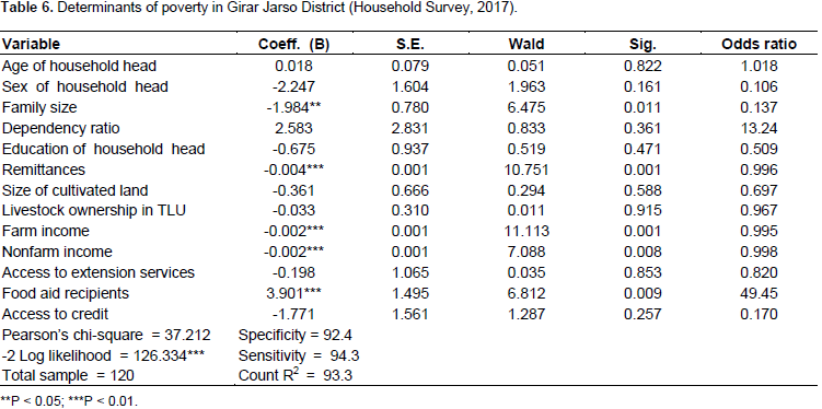
The estimated parameter, contrary to the earlier proposition revealed that family size has a negative significant (at p<5%) influence on household poverty. A unit increase in family size, ceteris paribus, leads the odds ratio of falling into poverty by a factor of 0.137. Family size as a covariate, negatively correlated with poverty is inconsistent with the findings of Bogale (2011) and Abebe (2017). The possible justification for this is existence of large number of economically active than non-active members of the community implying that there is a better demographic dividend. Recognizing that demographics have a dual impact on poverty raises the question of whether high fertility is an obstacle to poverty reduction or not. According to Bogale and Korf (2009), family size may have an ambiguous role in poverty status of rural households depending on the relative strength of size economies in consumption as against the diminishing return to scale.
As can be hypothesized, the coefficient of remittance is found to be negative, implying that the more households get remittance, the higher will be the tendency to be non-poor (at p < 5%). Interpretation of the odds ratio also indicated that probability of households in being poor decreases by a factor of 0.998 as households obtain one more unit of income from remittance. The possible reason here is that the society got a strong social network in which they send money to one another and an increase in number of educated household members’ migrants. Remittance is done in the area as part of their indigenous culture of helping each other deeds as community has a strong social cohesion. As expected, the model reveals that farm income shows a negative and significant effect on poverty (at p < 1%).
The negative sign indicates that when farm income earnings increases by one Ethiopian Birr, the likelihood of being non-poor, ceteris paribus, and increases by a factor of 0.995. The possible explanation is that those households who have sufficient access to farm income from sale of crop and livestock and their byproducts are more likely to be non-poor than those who do not earn enough farm income. Those households with more annual farm income have greater resilience or lower vulnerability to poverty. Majority of income earned goes to food expenditure improving accessibility of enough food and non-food expenditure. This result conforms to the findings of other studies (Abebe, 2017). Consistent with the earlier proposition, the model also reveals the important role of non-farm income in contributing to household poverty (at p<1%).
The odds ratio indicates that, other things being constant, the probability of the household to be poor decreases by a factor of 0.008 as the household earned one more unit of money from non-farm income. In this regard, households engaged in non-farm activities are better endowed with adequate income to purchase farm inputs and fulfill family needs and thus, get out of poverty. Additional income received from such activities to be one of coping mechanisms that could serve as a hedge against the future poverty. The higher income diversification implies the lower chances of being trapped in poverty. This negative and significant effect of non-farm income on poverty status was also confirmed by many researchers (Dawit et al., 2011; Babu and Afera, 2013; Megersa, 2015; Muhammedhussen, 2015). Although we hypothesized that food aid recipients have higher tendency to be non-poor, the model output revealed that it has positive association with household poverty (at p < 1%).
Receiving food aid increases the likelihood of being poor by a factor of 49.45. The study area is known to be drought prone and many households have been receiving food aid. Thus, the possible explanation for the unexpected output might be due to the existence of targeting inefficiency, dependency syndrome with repeated food aid for vulnerable households and disincentive effects. If food aid is not delivered in a timely manner, it could aggravate the cyclicality of prices associated with the harvesting and lean seasons due to inadequate storage. The most difficult issue has to do with the disincentive effects of food aid. The study further found that some households in the area even deplete their livestock resources in order to become poor and qualify for food aid. There is no statistically significant difference between the percentages of poor and non-poor participants in the programmes, and the socio-political connections of household apparently influence the likelihood of household participation (Calfa, 2010).