ABSTRACT
In order to spray herbicides accurately on targets, this study focused on spectral classification of weeds and crops for potential to rapidly detect weeds in crop fields. A 350 ~ 2500 nm FieldSpec-FR spectroradiometer was used to measure spectral responses of the canopies of the seedling vegetables, cabbage ‘8398’ and cabbage ‘Zhonggan 11’, and weeds, Barnyard grass, green foxtail, goosegrass, crabgrass, and Chenopodium quinoa, at five- and seven-week growth stages (WGS). First, the characteristic wavelengths (CW) were determined using Principal Component Analysis (PCA). Then, the plants were classified using Bayesian discriminant analysis with the reflectance of the CWs. The results of spectral analysis indicated that the different growth stages of cabbages had little influence on the spectral identification of cabbages and weeds. The eight CWs determined were used as the input to the model for Bayesian discriminant analysis to classify two varieties of cabbages and five weeds with the correct classification rate of 84.3% for model testing. When the two varieties of cabbages were considered as the same category, the correct classification rate was improved to 100%. It was concluded that Bayesian discriminant analysis could be used to identify weeds from seedling cabbages using leaf hyperspectral reflectance.
Key words: Weed identification, spectrum analysis, visible and near-infrared, Bayesian discriminant, seedling weed, seedling cabbage.
According to the research report from the United Nations Food and Agriculture Organization (FAO) in August, 2009, weeds should be regarded as farmers' No. 1 natural enemy. It was reported that according to a leading environmental research organization, Land Care of New Zealand, weeds cause about $95 billion every year in the lost food production at global level, compared with $85 billion for pathogens, $46 billion for insects, and $2.4 billion for vertebrates (excluding humans). Of the $95 billion, $70 billion are estimated to be lost in developing countries (FAO, 2009). In China, the crop yield losses annually caused by weeds sum up to about 10% of the gross grain output (Tang, 2010). Facing the severity of the crop losses caused by weeds, it is urgent to seek highly efficient methods for effective weed control. The chemical weeding method commonly adopted at present has provoked a lot of problems, such as excessive pesticide residues, growing number of pesticide-resistant weeds, destruction of ecological environment, and lower quality and safety of agricultural products (Thompson et al., 1991). Therefore, it is critical to have a method which could not only control the growth of weeds, but also decrease the use of herbicides, and hence prevent from excessive herbicide application. In order to minimize crop damage and environmental pollution, herbicides should be sprayed accurately on targets with appropriate dose.
Rapid access to the information of spraying targets is a critical process in precision chemical application. Many approaches to weed detection and identification have been reported in literatures, such as photoelectric detection technique (Biller, 1998; Andújar et al.,, 2011), ultrasonic detection technique (Andújar et al., 2012), remote sensing detection technique (Thorp and Tian, 2004), and image processing detection technique (Weis and Sökefeld, 2010; Christensen et al., 2009; Burgos-Artizzu et al., 2009; Piron et al., 2011), X-ray weed detection technique (Haff and Slaughter, 2009), and spectral weed detection technique (Vrindts et al., 2002; Sui et al., 2008). The image processing technique can detect the target’s profile and determine the coverage and amount of smart spray, but mostly this technique is still used in the laboratory instead of being used in field because of its poor stability, large amount of data processing, relatively slow response, and the high costs. In comparison, spectral detection has been widely used in real-time detection system because of its fast response, availability for non-contact detection, strong anti-interference, high reliability, low cost, simple and small configuration, and low power consumption. Many studies have focused on spectral classification of weeds and crops for potential to rapidly detect weeds in crop fields. Spectral sensors has been designed and widely used in real-time detection system in crop production, because they offer fast response, availability for non-contact detection, strong anti-interference, high reliability, low cost, simple and small configuration, and low power consumption (Wang et al., 2001; Rogalski, 2003). These sensors could be used to further study the spectral characteristics for classification of weeds and crops to realize fast and timely weed management in crop fields.
Koger et al. (2003) analyzed the hyperspectral reflectance of soybean, Ipomoea lacunosa, and soil at the two- and four-leaf stages of weed growth using wavelet analysis. For comparison, the raw spectral bands and principal components were used as discriminating features. For the two-leaf to four-leaf weed growth stage, the two features resulted in classification accuracies of 83 and 81%, respectively. Jurado-Exposito et al. (2003) distinguished sunflowers, wheat, and seven other seedling broadleaf weeds using near-infrared spectroscopy. It was found that the near infrared spectroscopy within 750 ~ 950 nm was able to identify these plants. Slaughter et al. (2004) distinguished Solanum weeds and tomato using the spectral reflectance in visible and near-infrared wavebands, narrow-band hyperspectral modeling, and discriminant analysis. It was found that the spectral absorbance data of weeds and tomatoes at the wavelength rang of 2120 to 2320 nm offered the best classification accuracy (100%), and narrow-band hyperspectral models of the data in the visible range also achieved good classification results (95%), while the broad-band models based on color information only provided 75% correct classification rate.
Thenkabail et al. (2004) studied how to select the optimum wavebands for classifying plants (shrubs and weeds) and crops (corn) in the range of 400 to 2500 nm waveband. It was found that 90% correct classification rate could be obtained by modeling using 13 to 22 wavebands selected from the original 168 wavebands using PCA and stepwise discriminant analysis, which accuracy was increased by 9 to 43% compared with modeling using ETM (Landsat Enhanced Thematic Mapper), plus brandband data. Piron et al. (2008) classified seven different weeds in carrot fields under artificial lighting conditions using a visible and near-infrared multispectral sensor, and found that overall correct classification rate was 72% when three optimal wavebands, 450, 550, and 700 nm were selected using the exhaust algorithm and used to establish the weed identification models. Mao et al. (2005) measured the spectral reflectance of wheat, shepherd's purse, and small quinoa in the wavelength range of 700 to 1100 nm using a Fourier transform infrared (FTIR) spectrometer, and extracted 7 characteristics wavelengths, 686, 708, 722, 795, 929, 956, and 1122 nm using stepwise discriminant analysis and achieved 97% correct identification rate through establishing the model of identifying wheat and weeds. Vrindts et al. (2002) measured the canopy reflectance of maize, sugarbeet, and seven weed species at 400 to 2000 nm. The spectral characteristics were also analyzed. Six wavelengths (555, 675, 815, 1265, 1455, and 1665 nm) at characteristic points in the spectrum were selected to derive the RVI. The STEPDISC and DISCRIM procedures in SAS were applied in the discrimination of crops (maize and sugarbeet) from weeds.
The classification result showed that crop and weeds could be recognized at an accuracy of higher than 97%. More than 90% of sugar beet and weeds could be identified correctly using a line spectrograph (480 to 820 nm) in classifying the plants. With the application of the spectral technique, Sui et al. (2008) developed the Weed Seeker sensor module to detect the presence of weeds by measuring the reflectance of weeds and bare ground. The module serves as a useful tool for locating weeds.
Karimi et al. (2006) used SVMs and NNs for weed and nitrogen deficiency detection in corn with non-imaging hyperspectral reflectance data as input. In an extensive approach, they uniquely identified and classified four weed management practices and three different nitrogen rates. The classification accuracy using SVMs was higher than with NN in this research project 69.2 versus 58.3%, respectively. Lopez-Granados et al. (2008) used the hyperspectral reflectance spectrum from 400 to 900 nm for the classification of late season grass weeds and wheat plants in a field study. Their approach using linear and nonparametric functional discriminant analysis and NNs has shown that, in general, a preliminary computation of most relevant PCs improves the classification accuracy. They concluded from their study that analysis in real time of high spectrally resolved images will be adequate to map grass weed patches in wheat. For practical implementation, Moshou et al. (2002) developed a weed species spectral detector based on neural networks with local linear mappings. A self-organized map (SOM) neural network achieved fast convergence and good generalization. The proposed method classified crops and different species of weed with high accuracy. Chen et al. (2009) measured the spectral reflectance of leaves of rice, cotton, Barnyard grass and Cephalanoplos indoors in the range of 350 to 2500 nm wavelength using a spectroradiometer and determined the characteristic wavelengths (CWs) using the stepwise discriminant method, and then classified these plants using the Discrim processing, a function of discriminant analysis in SAS statistical software (SAS Institute Inc., Carrey, North Carolina, the United States).
This study found that monocotyledons, like rice and Barnyard grass, could be accurately classified using the five CWs, 375, 465, 585, 705, and 1035 nm, in which the correct identification rate reached 100%; dicotyledons, like cotton and Cephalanoplos, could also be accurately classified using the three CWs, 383, 415, and 435 nm, in which the correct identification rate also reached 100%. The spectral reflectance of cabbages and weeds were measured in the 350 to 2500 nm band and preprocessed the data with different levels to improve the operation efficiency. All kinds of plants were classified using the Soft Independent Modeling of Class Analogy (SIMCA). While the selected 23 feature wavelengths were set as the input variables, the classification rate of the modeling set and the predicting set were respectively 98.6 and 100% (Zu et al., 2013a, b).
The objects of most of the previous studies were specific to crops like corn, wheat, rice, and cotton, but few to vegetables. The vegetables, especially dicotyledonous vegetables, are important economic crops in China, which are widely cultivated throughout the country with wide cultivated area and high inputs of labors. Therefore, weed identification in vegetable fields has considerable social and economic benefits and practical significance. Additionally, few of the previous studies were on whether the possible changes of spectral characteristics caused by the changing metabolism at the different growth stages of a crop would affect the consistency of spectral identification of crops and weeds during different growth stages.
For optimal results with minimal investment, weeds should be handled at seedling stage in crop fields (Li et al., 2007). Seedling weeds are sensitive to herbicides because plants are small and the tissues are young. Therefore, the seedling stage is the time for complete weed control. In the further growth stage, weed plants become large and their tissues are strong. Consequently, with the thickening of the waxy coat, it will be difficult for herbicide agents to penetrate the weed leaves and weed herbicide tolerance will be increased accordingly. As the result, the herbicide will be hard to take effect. This study was conducted on seedling weeds in the field with seedling cabbages.
In this study, two varieties of seedling cabbages, ‘No. 8398’ and ‘Zhonggan No. 11’, and five breeds of weeds, Barnyard grass, green foxtail, goosegrass, crabgrass, and Chenopodium quinoa, which are commonly-seen. Annual gramineous plants in cabbage fields with strong adaptability, wide coverage, fast multiplying, and inestimable harm to crops, were selected as the representatives of plants. The spectral reflectance of the plant canopies were measured in the wavelength range of 350 to 2500 nm at two seedling growth stages of the 35th (five-week growth stage (WGS)) and 50th days (seven WGS), respectively. The objectives of this study are (1) to determine CWs at which the spectral reflectances were sensitive to plant identification using the spectral data measured, respectively at five WGS and second WGS; (2) to establish the Bayesian discriminant model to classify two varieties of cabbages and five different weeds.
Experimental
Two varieties of cabbages used in the study were cabbage ‘No. 8398’ and cabbage ‘Zhonggan No. 11’, whose seeds were provided by the Institute of Vegetables, the Chinese Academy of Agricultural Sciences (Beijing, China). Five varieties of weeds were Barnyard grass, green foxtail, goosegrass, crabgrass, C. quinoa, whose seeds were provided by the College of Agronomy and Biotechnology, China Agricultural University (Beijing, China). The two varieties of cabbages and five kinds of weeds were planted in pots in a greenhouse of the Chinese National Engineering Research Center for Information Technology in Agriculture (Beijing, China) on 23 March, 2012. Each variety of plants was grown in 30 pots; therefore, the total number of the plant samples was 210 for the seven varieties of plants.
Data acquisition
The instrument for measuring spectral data was the ASD full range FieldSpec Pro. spectroradiometer (ASD, Inc., Boulder CO., USA). The measuring range of the spectroradiometer is 350 to 2500 nm. The spectral resolution is 1.4 nm in the range of 350 to 1000 nm and 2 nm in the range of 1000 to 2500 nm. The field of view (FOV) of the measuring probe is 25°.
The spectral data of the 210 pots of plant canopies were collected in the test field of National Engineering Research Center for Information Technology in Agricultural (Beijing, China) during 10:30 am to 14:30 pm on 28 April and 13 May, 2012, respectively, corresponding to two growing stages of the plants, five WGS and seven WGS.
The white reference board was measured for spectral calibration each 10 to 15 min depending on weather conditions. After each white reference measurement, the fiber-optic probe of the FieldSpec spectroradiometer was placed vertically above the plant canopy and measured the data. In order not to affect the reflectivity of the plants, the operator should dress dark. The spectroradiometer was set in the condition that an output datum was obtained from the average of ten measurements. The measured spectral data were converted to reflectance and then to ASCII text format using the function in the ASD ViewSpectro Pro. Software provided by ASD Inc. After being imported to Microsoft EXCEL spreadsheet, the text files were transformed to matrixes which were then transferred into the Unscrambler (CAMO software AS, Oslo, Norway) and SAS software for further data processing.
For data collection on 28 April, 2012, each pot of plants was measured for three times so that the total number of the obtained spectral data was 90 for each variety of plants (30 pots for each plant) and 630 for all the 7 varieties of plants. For the measurement on 13 May, 2012, each pot was measured for five times so that the total number of the collected spectral data was 150 for each variety of plant and 1050 for all the 7 varieties of plants.
In order to reduce the random errors which are always accompanied with the spectral signal in the process of data acquisition, the spectral data were averaged for each pot of plants, which resulted in 30 averaged spectral data for each plant respectively for the measurements on 28 April and 13 May.
Principal component clustering analysis
The clustering analysis of the spectral data of cabbages and weeds was conducted using the Principal Component Analysis (PCA) method after data preprocessing. For each of the plants, 20 sample data were randomly selected as the training sample set, the other 10 data as the testing sample set. In the Unscrambler software system, the full cross validation methods in PCA and Partial Least Square (PLS) were separately used to extract the principal components to build the plant classification models. The analysis process was started by extracting 20 principal components from the spectral reflectance data. Then, the outliers were repeatedly excluded by considering the spatial aggregation conditions and spatial position of all the sample points in scoring graphs of the results based on the principle of maximization of distance between the classes and minimization of distance within a class. The appropriate principal components were determined according to the cumulative credibility of each Principal Component (PC) and the classification model was re-built with clustering all the plants (Li, 2010).
Determination of characteristic wavelengths
In order to find out the CWs needed for identification of cabbages and weeds, the score of each PC, accumulative confidence level, and loading diagrams resulting from the former PCA and the relationship between PC and original wavebands expressed through loading graph should be analyzed. According to the loading graph of wavelength variable responding to the optimum PCs obtained from the former analysis, the wavelengths greatly (positive and negative) correlating with PCs were selected as the characteristic wavelengths sensitive to the identification of various of plants and with higher correlation for establishing the identification models. The loading coefficients of the selected wavelengths were used to reflect the importance of the wavelengths to the PCs.
Bayesian classification model
Bayes' theorem (Bayes 1764)
Mathematically, Bayes' theorem gives the relationship between the
probabilities of events
A and
B,
P(
A) and
P(
B), and the
conditional probabilities of
A given
B and
B given
A,
P(
A|
B) and
P(
B|
A). The form of Bayesian inference is mostly expressed as follows, provided that
P(
B) ≠ 0.
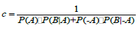
P(A|B) = [P(B|A)P(A)] / P(B)
Probability measures a degree of belief. Bayes' theorem then links the degree of belief in a proposition before and after accounting for evidence. For example, suppose somebody proposes that a biased coin is twice as likely to land heads than tails. Degree of belief in this might initially be 50%. The coin is then flipped a number of times to collect evidence. Belief may rise to 70% if the evidence supports the proposition.
For proposition A and evidence B, P(A), the prior, is the initial degree of belief in A. P(A|B), the posterior, is the degree of belief having accounted for B. The quotient P(B|A)/P(B) represents the support B provides for A.
The event
B is fixed in the discussion, and we wish to consider the impact of its having been observed on our belief in various possible events
A. In such a situation, the denominator of the last expression, the probability of the given evidence
B is fixed; what we want to vary is
A. Bayes theorem then shows that the posterior probabilities are
proportional to the numerator:
P(A|B) ∝ P(A)ï¹’P(B|A) (proportionality over A for given B).
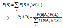
Further, if events A1, A2, …, are mutually exclusive and exhaustive, that is, one of them is certain to occur but no two can occur together, and we know their probabilities up to proportionality, then we can determine the proportionality constant by using the fact that their probabilities must add up to one. For instance, for a given event A, the event A itself and its complement -A are exclusive and exhaustive. Denoting the constant of proportionality by c we have:
P(A|B) = cï¹’P(A)ï¹’P(B|A) and P(-A|B) = cï¹’P(-A)ï¹’P(B|-A)
Adding these two formulas, we deduce that,
For that the extended form, often, for some
partition {
Aj} of the
event space, the event space is given or conceptualized in terms of
P(
Aj) and
P(
B|
Aj). It is then useful to compute
P(
B) using the
law of total probability:
Bayesian modeling
Using the eight CWs determined from the data at five WGS as the input variables, the discrimination model was built based on the Bayesian criterion and used to discriminate the cabbages and the weeds. In the process, 7 different plants were separately labeled using categorical variables as Y-8398 (cabbage 8398), ZG (cabbage Zhonggan 11), BC (Barnyard grass), GW (Setaria viridis), MT (crabgrass), NJ (Eleusine indica), and XL (C. quinoa). For each plant, two-thirds of the samples were randomly selected as the training group (140 samples) so that all the samples for the 7 plants were divided into two groups for training and testing, respectively. Then, using the data of categorical variables and 8 CWs, the discrimination model was built. In order to verify the reliability and robustness of the model, the other one-third of the samples (70 samples) were used as the testing group and the input of the model to classify the cabbage and weed samples.
Data observation
Further, the 30 averaged data were averaged for each variety of the plants. Figure 1 shows the averaged spectral reflectance curves for each of the plants. It can be seen that the curves are all the same as the typical healthy plant spectral reflectance curves. In the vicinity of 450 and 650 nm, the light of blue and red bands is absorbed by chlorophylls for photosynthesis, leading to two distinct absorption valleys. At 550 nm, the light of green light is partly absorbed by chlorophylls and partly reflected, forming a reflection peak. A steep slope at 700 to 800 nm demonstrates a sharp increase of reflectivity to form a high reflection platform. In the range of 800 to 1300 nm, the porous parenchyma tissue (spongy tissue) of plant leaves have always a very strong reflection to near-infrared light, creating a peak area of reflectance on spectral curves with the reflectance up to 40%. At about 1450 and 1950 nm, an apparent absorption valley is formed due to the cell sap, cell membranes, and absorbed vapor of the plant leaves.
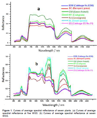
Particularly, it is shown in Figure 3 that for the spectral reflectance curves at the first WGS, the spectral reflectivity of green foxtail in the range of 700 to 1800 nm is obviously higher than other plants, while the spectral reflectivity of crabgrass comes to the next. In the range of 750 to 1100 nm, the reflectance of Barnyard grass is lower than other plants, while the spectral reflectivity of cabbages is modest and the spectral curves of two cabbages are almost superimpose. For the spectral curves at the seven WGS, the spectral reflectance curve of goosegrass is obviously distinct from other plants. It is seen that the curves of cabbages are relatively stable while the curves of weeds fluctuate dramatically, which could be a characteristic used to differentiate cabbages from weeds. In overall, there are some differences between the spectral curves of cabbages and weeds, but the spatial distributions of some samples overlap, which make it difficult to exactly distinguish the variety of each sample. In order to accurately classify cabbages and weeds, quantitative discriminant models should be established.
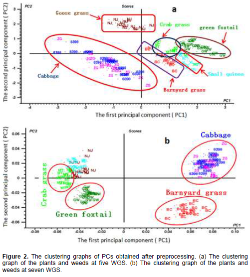
Clustering based on PCA
In the case of optimum preprocessing, the score plot of PC 1 and PC 2 of the training set is shown in Figure 2, in which the horizontal axis presents the score value of the first PC and the vertical axis is the score value of the second PC. It can be seen from Figure 2a that the data samples of cabbages mainly concentrate in the second and third quadrant, goose grass samples mainly in the upper area of the second quadrant, crabgrass and green foxtail samples in upper area of the first quadrant, Barnyard grass and C. quinoa principally around the horizontal axis in the fourth quadrant. It can be found from Figure 2b that cabbage samples closely distributing in the first quadrant show a good degree of aggregation which indicates that the two varieties of cabbages can be regarded as the same category. As well in a good degree of aggregation, all the Barnyard grass samples closely gather in the fourth quadrant and all the green foxtail in third quadrant. Although crabgrass samples distribute in both the second and third quadrant, the aggregating degree is still high. The samples of C.quinoa and goose grass loosely gather in the second quadrant. Therefore, it illustrates that PC1 and PC2 have better contribution to clustering cabbages and weeds. The synthetic method of PCA and clustering analysis can not only to a large extent reduce the data dimension but also greatly express the features of original data without losing the effective information.

Determining CWs
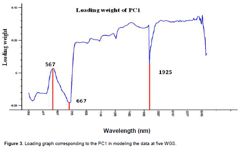
The loading diagrams corresponding to the optimum PCs obtained from spectral data processing at five and seven WGS are respectively shown in Figures 3 and 4. In the diagram, only the first PC is shown. In the loading diagrams, the horizontal coordinate represents the wavelength and the vertical coordinate is the load factor (that is, the correlation between wavelength and plant species) of each wavelength, wherein, the larger the absolute value of the corresponding load factor of a wavelength variable is, the stronger the correlation between the PC and the corresponding load factor is, and the more sensitive to the discrimination of the plant species.
It could be found from the loading diagrams that obvious crests and troughs present at some wavelengths and the rates of change of corresponding load factors appear as local maximum/minimum. These wavelengths are likely to play a decisive role in the identification of cabbages and weeds (Piron et al., 2011). Whereby, the corresponding CWs selected from the loading diagrams were 552, 567, 602, 607, 667, 715, 725, 1345, 1402, 1447, 1725, 1925, 1945, 1955, 2015, and 2072 for the five WGS plants and 425, 567, 667, 685, 745, 755, 1095, 1135, 1155, 1235, 1315, 1345, 1385, 1402, 1435, 1535, 1545, 1625, 1725, 1805, 1815, 1925, and 2030 for the seven WGS plants. The number of the CWs selected from the spectral data in the five and seven WGS was respectively 16 and 23.
Although the dimension of the data was already greatly reduced relative to the original data, the number of the band data is still relatively large for a practical instrumental design and development for agricultural use. Therefore, the selected CWs needed to be further optimized. The optimization process was to start with the first PC by sorting of wavelengths in terms of the absolute value of the corresponding load factors. Then, the wavelengths were further selected at which the absolute value of load was large and obvious crests and troughs were present in the loading diagrams. As the result, the selected CWs were 567, 667, 715, 1345, 1402, 1725, 1925, and 2015 nm for five WGS and 567, 667, 745, 1345, 1402, 1545, 1725, and 1925 nm at seven WGS (Table 1). In order to evaluate the effect of the selected CWs, the identification models were built using these CWs.
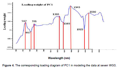
Among the each 8-CW set further determined respectively at two growth stages, just two of them were different as highlighted in bold in Table 1, which indicated that the change of the growth stage of cabbages and weeds had limited influence on the spectral features.
Bayesian classification
Based on the method mentioned in earlier, the discriminant functions of the classification models were obtained as follows in Equation 1, in which, the input variables (x1, x2, …, x8) are the eight CWs extracted from the data at the five WGS through PCA method.
BC = –49.89 + 75.11x1 + 976.62x2 – 247.88x3 + 8.52x4 + 184.98x5 + 360.82x6 + 115.39x7 – 464.08x8
GW = –68.91 + 1116x1 + 745.44x2 – 1112x3 + 677.47x4 – 436.09x5 + 222.38x6 + 44.97x7 – 216.67x8
MT = –45.98 + 213.48x1 + 668.17x2 – 309.73x3 + 300.99x4 + 149.24x5 – 24.16x6 + 114.15x7 – 285.32x8
NJ = –41.12 + 187.37x1 + 725.07x2 – 422.14x3 + 663.92x4– 98.88x5 – 338.86x6 + 127.71x7 – 76.97x8 (1)
XL = –93.59 – 3026x1 + 1839x2 + 1459x3 – 329.18x4 + 78.99x5 + 600.50x6 – 3.27x7 – 331.96x8
Y-8398 = –83.34 – 1803x1 + 1380x2 + 1344x3 + 39.46x4 – 148.77x5 – 358.52x6 + 87.37x7 + 218.22x8
ZG = –88.29 – 1874x1 + 1398x2 + 1432x3 – 118.03x4 – 87.21x5 – 211.36x6 + 54.09x7 + 172.79x8
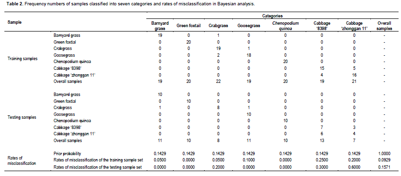
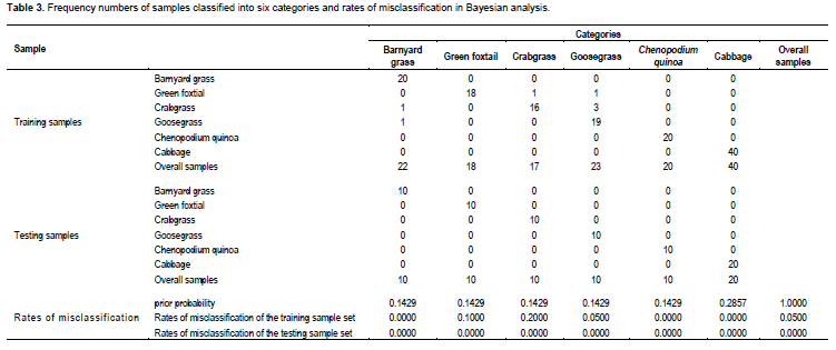
The frequency numbers of each training sample and the misclassified rates of the plants for 7 different plants discriminated into various categories are exhibited in Table 2.
In training data classification, five Cabbage ‘8398’ samples were misclassified as Cabbage ‘Zhonggan No.11’ and four ‘Zhonggan No.11’ as ‘ 8398’, which was because they are all cabbages with the identical internal structure and the similar pigment and appearance. Therefore, it is apparent that different varieties of cabbages can be considered in the same category. In addition, one Barnyard grass was misclassified as crabgrass, one crabgrass was misclassified as goosegrass, and two crabgrasses were misclassified as crabgrass, which is perhaps because they are all monocotyledonous weeds with similar internal structure and composition. Total of 13 samples in the training set were falsely classified and the misclassified rate is 0.0929, which is translated to 90.7% of the overall correct classification rate.
The classification results of the testing set showed that three Cabbage ‘8398’ were misclassified as Cabbage ‘Zhonggan No.11’ and six Cabbage ‘Zhonggan No.11’ were misclassified as ‘8398’. Moreover, one crabgrass was misclassified as goosegrass and one crabgrass was misclassified as Barnyard grass. Total of 11 samples were misclassified, therefore the misclassified rate is 0.1571. Then, the correct classification rate is 84.3%.
In order to verify the similarity of the spectral characteristics of different varieties of cabbages, cabbage ‘8398’ and ‘Zhonggan No.11’ were combined into one category. The 8 CWs which had been used earlier were still used as the input variables. All varieties of plants were labeled by categorical variables as GL (cabbage), BC (Barnyard grass), GW (S. viridis), MT (crabgrass), NJ (E. indica) and XL (C. quinoa). By repeating the previous process, the discriminant functions were obtained and shown as in Equation 2 and the classification results are shown in Table 3.
BC = –50.96 + 3412x1 – 3703x2 – 1259x3 + 1986x4 + 301.55x5 – 400.99x6 + 341.52x7 – 79.76x8
GW = –74.97 + 626.77x1 – 2181x2 – 1144x3 + 1988x4 + 246x5 – 27.37x6 + 89.15x7 – 30.93x8
MT = –53.05 + 2481x1 – 3611x2 – 906.51x3 + 1878x4+356.56x5–300.68x6+176.24x7–27x8 (2)
NJ = –42.19 + 3054x1 – 3533x2 – 1284x3 + 1688x4 + 280.05x5 – 146.62x6 + 75.17x7 – 1.76x8
XL = –72.26 – 5909x1 + 7404x2 – 1905x3 + 585.01x4 + 241.69x5 – 821.22x6 + 1190x7 – 356.42x8
GL = –73.44 + 4979x1 – 5095x2 – 744.15x3 + 2056x4 + 59.29x5 + 981.29x6 – 1335x7 + 374.43x8
From the results of the training set, for green foxtails, one was misclassified as crabgrass and one other as goosegrass; one crabgrass was misclassified as Barnyard grass and three were misclassified as goosegrass; one goosegrass was misclassified as Barnyard grass. Overall, the misclassified rate is 0.05, that is, the correct classification rate was 95%.
From the results of the testing set, all the samples were correctly classified therefore its correct classification rate was 100%. Compared with the previous correct classification rate from which the two varieties of cabbages were considered as two separate categories, the current correct classification rate had been greatly raised.
Using the ASD 350 to 2500 nm FieldSpec-FR spectroradiometer, the canopies of the seedling plants, cabbage ‘8398, cabbage ‘zhonggan’, Barnyard grass, green foxtail, goosegrass, crabgrass, and small quinoa, at five- and seven-week growth stages were measured. The results were concluded as follows:
(1) In terms of the load factors and the changing rate of the PCs, eight CWs which were sensitive to plant identification, were determined, respectively for the first growth stage of cabbages (five WGS) and the second growth stage (seven WGS). Among the 8 CWs for each growth stage, only two of them were different, which indicates that different growth stages of the cabbages have limited impact on the plant spectral characteristics for identification of cabbages and weeds.
(2) The corresponding spectral data of the 8 CWs determined from the data at the five WGS were used as the input variables of the Bayesian discriminant model to classify two varieties of cabbages and five different weeds. The correct classification rates for the training and testing sets were 90.7 and 84.3%, respectively. When the two varieties of cabbages were combined into the same category, the correct classification rates of the training and testing sets were improved to 95 and 100%, respectively, which indicates that different varieties of cabbages have similar spectral features to limit weed classification. Therefore, combining different varieties of cabbages as the same category could be effective to greatly improve the correct classification rates of weeds compared with the condition in which two varieties of cabbages were treated as different categories.
(3) The study results showed that Bayesian discriminant analysis could be used to identify weeds from seedling cabbages using leaf hyperspectral reflectance.
The authors have not declared any conflict of interests
REFERENCES
|
Andújar D, Àngela R, Fernàndez-Quintanilla C, Dorado J (2011). Accuracy and feasibility of optoelectronic sensors for weed mapping in wide row crops. Sensors 11:2304-2318.
Crossref
|
|
|
|
Andújar D, Weis M, Gerhards R (2012). An ultrasonic system for weed detection in cereal crops. Sensors 12:17343-17357.
Crossref
|
|
|
|
|
Bayes T (1764). An essay toward solving a problem in the doctrine of chances. Philos. Trans. R Soc. London 53:370-418.
Crossref
|
|
|
|
|
Biller RH (1998). Reduced input of herbicides by use of optoelectronic sensors. J. Agric. Eng. Res. 71:357-362.
Crossref
|
|
|
|
|
Burgos-Artizzu X P, Ribeiro A, Tellaeche A, Pajares G, Fernández-Quintanilla C (2009). Improving weed pressure assessment using digital images from an experience-based reasoning approach. Comput. Electron. Agric. 65:176-185.
Crossref
|
|
|
|
|
Chen S, Li Y, Mao H, Shen B, Zhang Y, Chen B (2009). Research on distinguishing weed from crop using spectrum analysis technology. Spectrosc. Spec. Anal. 29(2):463-466.
|
|
|
|
|
Christensen S, Søgaard H, Kudsk P, Nørremark M, Lund I, Nadimi E, Jørgensen R (2009). Site-specific weed control technologies. Weed Res. 49:233-241.
Crossref
|
|
|
|
|
FAO (2009). The lurking menace of weeds. Available at:
View
|
|
|
|
|
Haff RP, Slaughter DC (2009). X-ray based stem detection in an automatic tomato weeding system. In: ASAE Annual Meeting. Paper Number: 096050.
|
|
|
|
|
Jurado-Expósito M, López-Granados F, Atenciano S, GarcíA-Torres L (2003). Discrimination of weed seedlings, wheat (Triticum aestivum) stubble and sunflower (Helianthus annuus) by near-infrared reflectance spectroscopy (NIRS). Crop Prot. 22(10):1177-1180.
Crossref
|
|
|
|
|
Karimi Y, Prasher OS, Patel RM, Kim HS (2006). Application of support vector machine technology for weed and nitrogen stress detection in corn. Comput. Electron. Agric. 51(1-2):99-109.
Crossref
|
|
|
|
|
Koger CH, Bruce LM, Shaw DR, Reddy KN (2003). Wavelet analysis of hyperspectral reflectance data for detecting pitted morningglory (Ipomoea lacunosa) in soybean (Glycine max). Remote Sens. Environ. 86(1):108-119.
Crossref
|
|
|
|
|
Li Z, Rao H, Wang Y, Ji C (2007). Status quo and advance on research of variable- rate spraying technology. J. Northeast Agric. Uni. 38(4):563-567.
|
|
|
|
|
Li G (2010). Research on discrimination of varieties of invasive weeds based on visible and near-infrared spectroscopy. Dissertation of Zhejiang University, Hang Zhou, China. (In Chinese with English abstract)
|
|
|
|
|
Lopez-Granados F, Pena-Barragan JM, Jurado-Exposita M, Francisco-Fernandez M, Cao R, Alosno-Betanzos A (2008). Multi spectral classification of grass weeds and wheat (Triticum durum) using linear and nonparametric functional discriminant analysis and neural networks. Weed Res. 48(1):28-37.
Crossref
|
|
|
|
|
Mao W, Wang Y, Zhang X (2005). Spectrum analysis of crop and weeds at seedling. Spectrosc. Spec. Anal. 25(6):984-987.
|
|
|
|
|
Moshou D, Ramon H, De Baerdemaeker J (2002). A weed species spectral detector based on neural networks. Precis. Agric. 3(3):209-223.
Crossref
|
|
|
|
|
Piron A, Leemans V, Kleynen O (2008). Selection of the most efficient wavelength bands for discriminating weeds from crop. Comput. Electron. Agric. 62(2):141-148.
Crossref
|
|
|
|
|
Piron A, van der Heijden F, Destain MF (2011). Weed detection in 3D images. Precis. Agric. 12:607-622.
Crossref
|
|
|
|
|
Rogalski A (2003). Infrared detectors: status and trends. Prog. Quant. Electron. 27(2):59-62.
Crossref
|
|
|
|
|
Slaughter DC, Lanini WT, Giles DK (2004). Discriminating weeds from processing tomato plants using visible and near-infrared spectroscopy. Trans. ASABE 47(6):1907-1911.
Crossref
|
|
|
|
|
Sui R, Thomasson JA, Hanks J, Wooten J (2008). Ground-based sensing system for weed mapping in cotton. Comput. Electron. Agric. 60(1):31-38.
Crossref
|
|
|
|
|
Tang J (2010). Research on Weed Detection and Navigation Parameters Acquisition of Pesticide Spraying Robot. Dissertation of North-west Agriculture and Forestry University, Yang Ling, China. (In Chinese with English abstract)
|
|
|
|
|
Thenkabail PS, Enclona EA, Ashton MS, Meer BVD (2004). Accuracy assessments of hyper spectral waveband performance for vegetation analysis applications. Remote Sens. Environ. 91(3):354-376.
Crossref
|
|
|
|
|
Thompson JF, Stafford JV, Miller PCH (1991). Potential for automatic weed detection and selective herbicide application. Crop Prot. 10(4):254-259.
Crossref
|
|
|
|
|
Thorp K, Tian L (2004). A Review on Remote Sensing of Weeds in Agriculture. Precision Agriculture. pp. 5477-508.
Crossref
|
|
|
|
|
Vrindts E, De Baerdemaeker J, Ramon H (2002). Weed detection using canopy reflection. Precis. Agric. 3(1):63-80.
Crossref
|
|
|
|
|
Wang N, Zhang N, Peterson DE, Dowell FE (2001). Design of an optical weed sensor using plant spectral characteristics. Trans. ASAE 44(2):409-419.
Crossref
|
|
|
|
|
Weis M, Sökefeld M (2010). Precision Crop Protection - the Challenge and Use of Heterogeneity; Springer Verlag: Dordrecht/Heidelberg/London/New York. Detect. Ident. Weeds 1:119-134.
Crossref
|
|
|
|
|
Zu Q, Zhao C, Deng W, Wang X (2013a). Research on discrimination of cabbage and weeds based on visible and near-infrared spectrum analysis. Spectrosc. Spec. Anal. 33(5):1202-1205. (In Chinese with English abstract)
|
|
|
|
|
Zu Q, Deng W, Wang X, Zhao C (2013b). Research on spectra recognition method for cabbages and weeds based on PCA and SIMCA. Spectrosc. Spec. Anal. 33(10):2745-2750.
|
|