Agricultural statistics indicate that per capita food production in Rwanda is declining (Minecofin, 2003a; RADA, 2005; NISR, 2008). This trend is putting at stake the food security of the rural and urban poor. Rwandan agriculture is not able to meet its population’s food needs with the national production.

 

Land degradation is a serious problem which contributes to the low and declining agricultural productivity and consequently to food insecurity. Land degradation can be defined in terms of loss of actual or potential productivity as a result of natural or human factors (Anecksamphant et al., 1999). Soil erosion  and soil mining are believed  to

be the most important causes of land degradation in Rwanda with a soil loss of 50 to 400 tons per hectare per year depending on location (Mugabo, 2005). Some slopes are totally degraded by erosion and no production is possible without restoring fertility. In addition, Rwandan soils have a very low organic matter content and weak soil fertility potential except for the marshy and volcanic soils (Gecad, 2004). Furthermore, land scarcity due to the high population density is limiting the option to  extend agricultural land size. In Rwanda, the biophysical causes of land degradation are relatively well known, but less is known about the economic impact of land degradation on farming activities. Very little modelling analysis exists at farm level on the economic consequences of land degradation (Byiringiro and Reardon, 1996; Clay et al., 1998; Musahara, 2006).

 

Rwanda’s population, which is made up mostly of subsistence farmers, has quadrupled during the last 50 years. At present, Rwanda has 9.3 million inhabitants with a density of 380 inhabitants/km². The average size of a family farm is 0.76 ha (Minagri, 2004). If the human reproduction rates are not slowing down, the population will double by 2030 (Kinzer, 2007), with dramatic consequences for natural resources and food security. Thus, it is important to balance the increasing population with the limited available land, and ensure food security.

 

The new land law put in place by the Rwandese government stipulates that, under its article 20, landholdings less than one hectare (ha) are deemed insufficient for effective and efficient agricultural exploitation (Minerena, 2005). Therefore, the Rwanda government prepared to use the land law as one of the drivers of agricultural reform, notably through the provision on land consolidation and minimum land holdings. The farm households whose land is less that 1 ha would have difficulties to register their land (Huggins, 2012). The land law and land policy tend to stimulate farm households whose landholdings are less than one hectare to consolidate their land, but those who are reluctant to comply to the land law and land policy are vulnerable to confiscation of their land (Huggins, 2012; Pottier, 2006). This ruling follows a recommendation made by the Poverty Reduction Strategy paper (Minecofin, 2003b): “households will be encouraged to consolidate plots in order to ensure that each holding is not less than 1 ha. This will be achieved by the family cultivating in common rather than fragmenting the plot through inheritance”.

 

Decisions on land use are basically made by heads of farm households. As in many other developing countries, a farm household system in Rwanda concerns production (of crops and livestock), off-farm activities and consumption (of food, other basic needs and some leisure). A major characteristic is the non-separability of production and consumption decisions. The allocation of productive resources and the choice of activities could affect land degradation and subsequently food security. It is assumed that farm households are rational in pursuing certain meaningful objectives which guide their behaviour (Upton, 1996; Anderson, 2002; Woelcke, 2006; Laborte et al. 2007; Laborte et al., 2009). However, the decision-making process is restricted by the range of possible alternative activities that can be undertaken by farm households and constraints imposed by limited resources availability and other external conditions like agricultural and/or environment policies (Senthilkumar et. al, 2011).

 

To understand the complex relations at farm level between technical, ecological and economic components, there is a need to combine information from biophysical and social sciences (Kruseman, 2000). Bio-economic modelling is at the interface of biophysical and social sciences, enabling the accommodation of biophysical data in economic analysis (Kanellopoulos et al., 2010; Louhichi et al., 2010).

 

In developing countries, many studies have made use of bio-economic farm models and there is growing interest for its application (Jansen and Van Ittersum, 2007). However, little modelling analysis at farm household has been conducted in subsistence or semi- subsistence farming. Barbier (1990), Cárcamo et al. (1994), Barbier and Bergeron (1999) and Louhichi et al. (1999) evaluated the economic nature of land degradation and estimated net returns from erosion control. Van Keulen et al. (1998), Kruseman and Bade (1998), Kuyvenhoven et al. (1998), Ruben et al. (1998), Struif Bontkes and Van Keulen (2003) assessed different sustainable technologies to improve farm household income and soil fertility. Dorward (1999) investigated the conditions under which peasant farm household models may need to allow embedded risk. Anderson (2002), Mudhara et al. (2002), Thangata et al. (2002) examined the options for improving household food security for small-scale farms.

 

Modelling farm households might bring some insights into the ongoing debate on land and family planning reforms and the potential impacts of soil erosion. So far no modelling studies in sub-Saharan countries have incorporated at the same time soil erosion, soil fertility, soil quality and food consumption in terms of energy and proteins, risk, labour, land, cash and credit availability in their economic evaluation of crop production for farms.

 

The objectives of this paper are:i) to develop a general bio-economic model capable of analysing the impacts of family planning, land consolidation and soil erosion on farm production and food security in Rwanda; ii) to apply the bio-economic model for a typical farm in Rwanda.

 

The remainder of this paper is structured as follows. The next section describes the study area and the farm household model. Next, data and application of the model for a typical farm are presented. This typical farm household has available resources that are the average of farm types distinguished in (Bidogeza et al., 2009).

 

This is followed by the presentation of the modelling results regarding food security, technical and economic results for the typical farm. The outcomes of the farm household model are compared with observed farm household data; and the effects of family and land size changes on food security, income and soil loss results are determined and discussed. Thereafter follow the conclusions.

Area of study and typical farm

 

The area of study is in Umutara, a former province located in the eastern part of Rwanda, approximately 180 km from Kigali along the main tarmac road between Kigali and Kagitumba (border with Uganda). It has a border with two countries, Uganda in the north, and Tanzania in the southeast. The tarmac road and the geographical position of Umutara imply that the market access is fairly good.

 

Most inhabitants of Umutara are former refugees who arrived from Tanzania and Uganda after the genocide which ended in 1994. When they returned to Rwanda, Umutara was chosen for their resettlement. The increasing population puts a high pressure on natural resources of the province, and different land uses often compete for the same piece of land.

 

Umutara province belongs almost entirely to the agro-climatic zone of the Central Bugesera and the Savannahs of the East, which is the driest agro-climatic region of Rwanda. The annual precipitation is quite variable in the region and is on average lower than 1000 mm (Sirven et al., 1974). The irregularity of the precipitation is a frequently stated problem for Umutara. The climate of Umutara is bimodal (Fleskens, 2007), with two growing seasons annually. The agricultural activities for one season referred to as B last from January to June, and agricultural activities for the other season referred to as A take place from July to December.

 

The pedology of Umutara is quite diverse, notwithstanding that it is only a small area. Two types of soils are dominant in Umutara: Inceptisols and Oxisols (USDA, 1999), mostly located on gentle (2-6%) and moderate (6-13%) slopes, respectively. These land types are covering 60% of the total soil in Umutara province, respectively 40% for Oxisols and 20% for Inceptisols (GhentUniversity, 2002). The chemical fertility of Oxisols is poor; weathered minerals and cations retention by mineral soil fraction is weak, while Inceptisols have a satisfactory chemical fertility and contain at least some weathered minerals in silt and sand fraction (FAO, 2001). Despite of the low fertility of the soils, small-scale farmers maintain soil fertility and reduce soil erosion by using low input systems such as crop rotations,  organic  fertilisers and few of them also use some chemical fertilisers. However, these land management strategies are not suficient for a sustainable farming.

 

With respect to the importance of the different crops cultivated in the region: 33% of the cultivated land is occupied by cereals, followed by tubers (29%), leguminous crops (21%) and bananas (15%) (Minagri, 2002).

 

The farm household analysed in this paper is typical for the province. Important socio-economic variables used to characterise the typical farm household were average farm data at regional or national level derived from the literature and field survey (Kinzer, 2007; Loveridge et al., 2007; Strode et al., 2007; Ansoms and McKay, 2010).

 

Model specification and data used

 

General structure

 

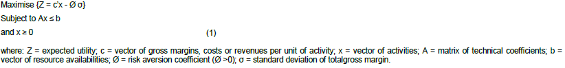
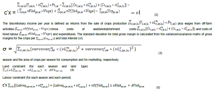
The basic structure of the bioeconomic farm household model is shown in Equation (1). It has the mathematical form of a quadratic programming model (Hazell and Norton, 1986):            

 

 

The model presented here is a quadratic programming model with a time span of one year (two seasons). The expected utility is the objective function and this is maximized. The farmer is assumed to maximise expected utility which is defined as discretionary income minus the risk premium. Discretionary income is defined as income available for spending after essential expenses have been made (Castano, 2001; Laborte et al., 2009). The most important essentials include clothes, taxes, medication, school fees, kitchen ustensils and food ingredients.

 

Activities include crop production for home consumption, crop production for sale, off-farm activities, hiring labour, family expenditures, borrowing credit. Major constraints include land, labour in three different periods per season, rotations, available cash, maximum credit, food consumption requirements, soil loss and soil organic matter.

 

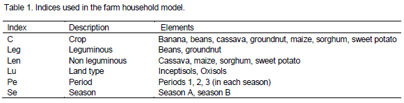
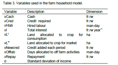
The major activities and constraints are summarized bythe Equations (2) to (14). For the description of the indices, coefficients and variables see Tables 1, 2 and 3, respectively.

 

 

 

 

 

 

The software used for optimization of the quadratic programming farm household model is General Algebraic Modelling System, version 22.6 (GAMS) with the solver CONOPT.

 

Sources of data used

 

In 2004 and 2005 data were collected in  Umutara  province  by  the National Institute of Statistics of Rwanda, in the framework of a national agricultural farm survey held twice annually. This farm survey database can be obtained from the authors upon request. In addition, a small survey was conducted in October, November and December 2007 through interviews in order to collect information supplementary to the national farm survey. For the latter survey, farm households were asked questions about family expenditure and income, crops and rotations, production costs and output prices, labour use and costs, market availability. Supplementary information related to coefficients of the current farming were estimated from literature (MCDF, 1984; Birasa et al., 1990; Minagri, 1991; Ghent university, 2002; CPR, 2002; Minagri, 2002; Zaongo et al., 2002; Van Ranst, 2003; CIRAD, 2004 and Minagri, 2006). These coefficients are estimated under low input systems. Low inputs are defined as no significant use of purchased inputs such as artificial fertilizers, improved seeds, pesticides or equipment. Input and output prices in the region were derived from the database on the market prices list provided by the Minagri (2007). Data to generate many of the coefficients for soil characteristics of the region were obtained from the natural resource database hosted by the “Carte Pedologique” Unit at the Ministry of Agriculture (Birasa et al., 1990).

 

Activities

 

Farm household activities consist mainly of crop production, off-farm activities and hiring in labour or working as farm labour on other  farms.  Livestock is  not  a  major  activity  for  the  farm  type considered. Major food crops in Umutara include beans, groundnut, maize, sorghum, cassava, sweet potatoes, and banana. Crop activities in the model are production for sale and production for home consumption, since farm households consume a large part of their own products and sell what remains. Thus, we have assumed in the farm household model that any production above subsistence requirements will be sold.

 

All crop activities are defined at the level of annual cropping systems except banana and cassava, which are perennial crops. Subsequently, each of the perennial crops is assumed to have equal land area in the two growing seasons.

 

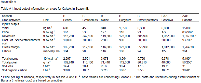
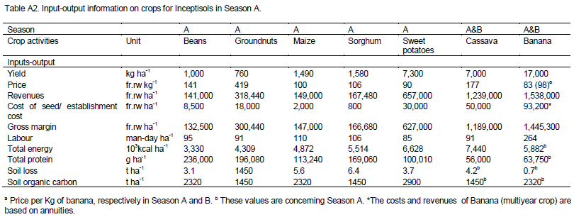
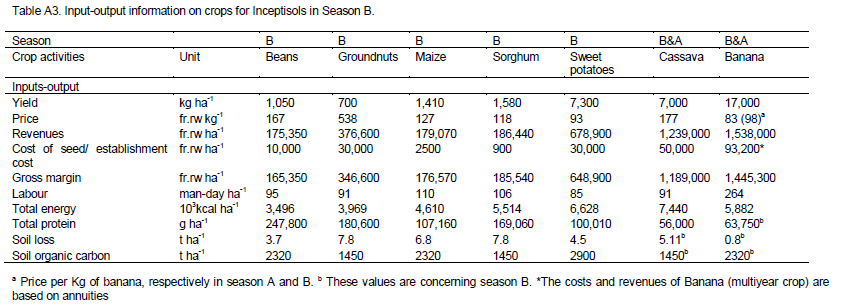
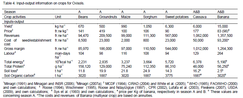
Table 4 presents a summary of input-output information for the different crop activities for season A and for Oxisols. Input-output information for the other season and the other soil type is provided in Appendix A.

 

 

Off-farm activities are important for the household systems in Rwanda. Off-farm activities represent an alternative source of income which must be taken into account when maximizing the farm income. Available off-farm activities  concern  informal  sector  work  and  include activities such as running small businesses, hiring out labour or working as vendor in the market etc. The family labour that can be devoted to off-farm activities depends on the available labour of the head of the household since he is the one who is mostly involved in these activities. However, off-farm opportunities are scarce in these rural areas. In our farm household model, we have assumed that a head of household can devote at most 50% of the available time for labour to off-farm activities. The daily wage received by the head of household for participating in off-farm activities is 400 fr.rw. This is the average daily wage for agricultural and informal non agricultural labour in eastern region (Strode et al., 2007).

 

Hired labour can be used in addition to farm household labour when cash is available. Hence, hired labour and farm household labour may be regarded as perfect substitutes. The wage of hired labour amounts to 400 fr.rw per man-day (Strode et al., 2007).

 

Borrowing can be seen as an option to supplement insufficient cash in order to finance seeds, hired labour, school fees, etc. Financial institutions could be important sources of  credit  facilities.  However,  in  practice  farmers find it quite difficult to acquire credit from these institutions due to the lack of collateral. Instead, credit can be obtained from informal sources like “credit club”, the primary source of credit in Umutara. Loans plus interest must be repaid at the end of the cropping season. Interest is paid at the rate of 10% per month  depending on the “credit club” to which a farm household has subscribed. Although that credit can be available, it is constrained by a credit limit .

 

Constraints

 

Land available for the representatative farm household is based on the average farm size in the eastern region, which is 0.7 ha (Loveridge et al., 2007). Crops may be grown on two soil types Oxisols and Inceptisols.

 

Labour requirements for crop activities (Table 4) vary depending on crop development stage. Most of the field operations on crops (land preparation, planting/sowing, crop maintenance, hand weeding and harvesting) have to be performed during a particular period of the season. Thus, each  season  is  divided  into three periods of two months. Small-scale farm households typically use family labour. Composition of the household determines labour capacity. The labour capacity of an adult farm household member is 100%, while children (10-18 years) and adults over 65 years of age are assumed to have 50% working availability. The available farm family labour may be subject to fluctuations over the year.

 

In fact, for school-going adolescents, labour contributions vary, depending on whether they live at home during school year. Additionally, children also contribute to the farm labour force during their vacations in April, July, November and December. We assume that available labour that can be allocated to activities is equivalent to 5 days per week per adult. However, 1 day per week per adult is substracted since farm households allocate labour to other necessary activities such social and household activities (e.g. firewood and water collection). The total labour requirements for crop production should be met by farm household labour and hired labour.

 

Rotation restrictions are set for individual crops for agronomic reasons. Crop rotations can be very important for pest and disease control, for maintaining soil fertility and reducing soil erosion. Seasonal crop rotation practices are widely adopted by farmers throughout the country. Crop rotations are incorporated in the model as strict equality constraints and imply that areas of the crops in the rotation are equal. The most frequently adopted rotations for the region are cereals-leguminous (that is, maize and sorghum with beans and groundnut) and tubers-leguminous (that is, sweet potatoes with beans and groundnut).

 

Cash is required to finance expenses of crop production during each cropping season and is a major constraint for small-scale farm households. These expenses include family expenditures, purchase of seeds and hiring labour. Cash is also needed for family expenditures. Cash is available from farm household’s own savings made in the previous harvesting season. Moreover, cash may come from off-farm activities and credit. Credit limits set a limit to the amount of credit to be lent to a farmer. The limit varies from 5,000 Fr. Rw to 50,000 Fr. Rw depending on the wealth of the farmer. In the model, we assumed a credit limit of 10,000 fr.rw (Bidogeza et al., 2009).

 

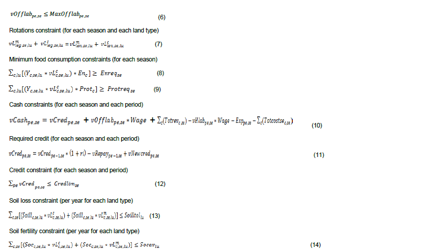
Food consumption constraints in the model reflect the need of the household to first secure the household food requirements since the primary objective of small-scale farmers in Rwanda is to provide their families with adequate food . Food purchases have not been considered in  model  since  the  food  consumption  is  mainly from the farm’s food production. Small-scale farmers can hardly buy food. Consumption constraints are specified to guarantee minimum energy (in kilocalories) and proteins (in grams) per season. The minimum food requirements are obtained from the World Health Organization (WHO) recommendation level of energy and proteins per person (Table 5). 

 

 

Soil organic carbon (SOC) is one of the key factors that affect agricultural production, nutrient availability and soil stability (Tang et al., 2006), particularly in highly weathered Rwanda soils where organic matter is the major source of nutrients. SOC is a dynamic property of soil, not a static one (Cooperband, 2002). The crop requirements for SOC are derived from Sys et al. (1993). The right hand side of the SOC constraint specifies its tolerance value below which yields begin to decrease (Barbier, 1998). Arshad and Martin (2002) suggested that for SOC a decrease of 15% over the average or the baseline value seems reasonable to use as critical value.The baseline SOC values considered are the organic carbon content of the two soil types for a soil depth of 1m (Ghent University, 2002).

 

Soil loss above certain limits will lead to the degeneration of soil reserve and soil fertility resulting in the destruction of the usable agricultural land. The farm household model takes soil loss into consideration as a constraint. Soil loss values are required for each crop activity. These values are incorporated into a soil loss constraint for each of two land types, respectively Inceptisols and Oxisols. The Wischmeier’s model (Universal Soil Loss Equation) is used to calculate the soil loss coefficients (Wischmeier, 1995). The model predicts gross soil loss per unit of land as:

 

                                                              (15)

 

where A is the estimated soil loss in tons per hectare. R is the rainfall erosivity calculated based on the total kinetic energy of the rainfall and the maximum rainfall intensity over a continuous 30 min period. It represents the potential erosive risks for a particular region. R values have been derived from Equation (16) and are obtained from measurements in a region of Uganda which has close similarities with Umutara (Lufafa et al., 2003).

 

                                                          (16)

 

In formula (16) Pr is the seasonal precipitation (mm). K is soil erodibility and represents soil resistance. K is a function  of  texture, organic matter, permeability and soil structure. K values for Inceptisols and Oxisols are respectively 0.20 and 0.25 (Roose and Ndayizigiye, 1997; Henao and Baanante, 2006; Fleskens, 2007). L*S represent hillslope length and steepness, and reflects the effect of topography on soil loss rates at a particular site. Values used for Inceptisols with slope of 4% and Oxisols with slope of 9% are respectively 0.42 and 1.3 (Roose, 1994). C is the land use and land cover factor and expresses effects of surface cover and roughness, soil biomass, soil-disturbing activities on rates of soil loss at particular sites. Values used are obtained from Lewis (1988; cited by Fleskens, 2007). Banana has the lowest C-value of 0.04, while sorghum has the highest C-value of 0.45. P is management practice and expresses the effects of supporting conservation practices, such as contouring, buffer strips, terracing, etc. on soil loss at a particular site. When no erosion control practice is used, P equals 1. Planting crops with dispersed trees could be attributed a P value of 0.6, use of grass strips lowers this to 0.4 and grass strips with hedgerows P to 0.1. Thick mulching also has a P of 0.1 (Fleskens, 2007 and Roose, 1994).

 

The right hand side of the soil loss constraint specifies the soil loss tolerance. The concept of soil loss tolerance is defined as the maximum acceptable soil loss from an area which will allow a high productivity to be maintained for a long period of time. In the model, soil tolerance values used for Oxisols and Inceptisols were derived from Pretorius and Cook (2002), 12 t ha^-1 yr^-1 and 16 t ha^-1 yr^-1, respectively. Pretorius and Cook (2002) have assigned soil tolerance values to soils depending on their root penetration depth. The Oxisols have generally steeper slopes and lower soil depth, while Inceptisols are on gentle solpes and deeper soils.

 

Inclusion of risk in the farm household model

 

It is important to account for risk in any agricultural productive activity (Hardaker et al., 2004; Anderson and Dillon, 1992). Risk is defined as a measure of the effect of uncertainty on the decision-maker (Upton, 1996). Farm households in Rwanda are facing an unstable income from season to season due to unpredictable rainfall and fluctuations of market prices. Most small farmers typically behave in risk-averse ways, they are willing to forgo some expected income for a reduction in risk (Acs et al., 2009). Ignoring risk-averse behaviour in farm household models may lead to results that are unacceptable to the farmer, or that have little relation to the decisions he actually makes.

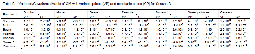
From Equation (1) risk is explicitly incorporated in the farm household model. The risk is calculated following a quadratic programming approach (Hazell and Norton, 1986). This method computes the standard deviation from the variance-covariance matrix and the level of the stochastic activities. Since seasonal fluctuations in farm prices and rainfall have a large effect on farmers’ income, risk has been calculated for two types of production activities: home consumption and market. To compute risk for home consumption, we use gross margin with  constant prices, while gross margin with variable prices is used to compute market risk. Data from six years are used to determine the variance and covariance matrix. This is refered to in Table 6 for Season A. The variance and covariance matrix table for Season B is shown in Appendix B.

 

 

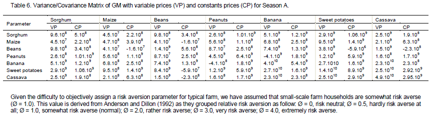
The risk aversion coefficient of 1 is within the range of values reported by Senkondo (2000), that is, -0.98 and 2.64 with an average value of 0.774 for the situation when the farmer has inadequate food stocks, which is a situation quite similar for the typical farm household in Rwanda.

 

Set up of the calculations

 

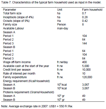
Calculations are made for a typical farm household on Oxisoils and Inceptisoils for the two growing seasons of a year. Table 7 shows some specific farm characteristics for the representatative farm household considered in the model. The farm household is composed of one adult male, one adult female, two kids under 10 years old and four children are of age 10-18. This family size follows from the average national rate of birth with six child per woman (Kinzer, 2007). The household is supposed to benefit of the labour from the children while they have vacation. Consequently, the available labour within the household fluctuates within the year as it can be seen from the Table 7. Average yearly expenditures of the typical farm household are estimated on the basis of national value representing the consumption poverty line per adult equivalent per year. That value is estimated at 64,000 Rwandese francs per adult equivalent per year (Ansoms and McKay, 2010). The farm household is assumed to have two adults (the head of household and his wife). The children are added to this adult equivalent. For the cash availability, we assume that the farm houshold has a cash of 5,000 Fw.Fr at the beginning of the year (Bidogeza et al., 2009).

 

 

Subsequently, the results from the typical farm household model are compared with actually observed values. Lastly, additional calculations are made with the model to examine the effects of the land area and family size on food security , income and soil loss results. Therefore, the farm household model is optimized with nine different combinations of land area and family size. Three households with a family size of five, eight, and ten persons are combined each, with a land area of 0.5, 0.7 and 1 ha, respectively. The household size of five, eight and ten reflect respectively: the Government's policy on family planning which encourages families to have at most 4 children per woman (Solo, 2008); the current average family size (about 8) and a rather high household size, also often encountered in Rwanda. The land areas embody, respectively the possible  future,  the  actual,  and  the  minimum  recommended

land size.

Calculations have been made first to determine the optimal farm plan for the typical farm.

 

Technical results

 

The optimal cropping plan for the typical farm is presented in Table 8. A large proportion of land is allocated to banana, beans, sweet potatoes and sorghum which reflects the food habits in Umutara province. Banana and sweet potato have higher calories per hectare while beans have the highest level of proteins per hectare. Banana covers a much larger proportion (47%) of the land in the optimal farm plan than other crops because of its high calories per hectare. In addition, banana protects well the soil since it causes less soil loss. Sweet potato also has high yield of calories per hectare but, because of the high soil loss  rate  compared to banana, a smaller land area is allocated to sweet potato than banana. Beans are produced to a relatively large extent (20%) because of its highest level of proteins. A small proportion of the available land is allocated to sorghum and groundnut to supply additional calories and proteins and secure the nutritional requirements of the farm household.

 

 

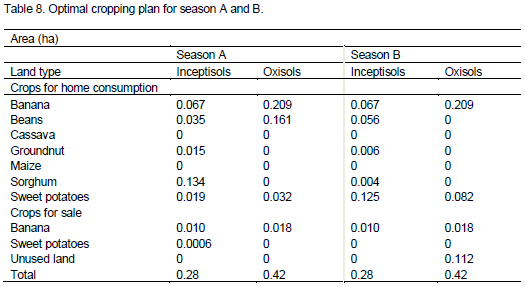
From the model results, both nutritional requirements and soil loss are binding constraints. However, soil loss is restricting only on marginal land (Oxisols). Banana and beans cause less erosion compared to other crops. This explains why they are grown mostly on marginal land (70%).

 

Cassava is not considered in the optimal farm production although it has the highest yield of calories per hectare. The model considers that an optimal plan including cassava is too risky since it has a higher variability of production and prices compared to other crops.

 

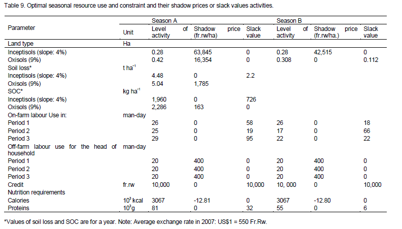
Technical results for fixed resources, specifically land, on-farm labour and off-farm labour are shown in Table 9. The area under Inceptisols is fully used in both seasons, whereas the model leaves 0.112 ha of the area under Oxisols unexploited in season B. This is because of constraining soil loss and SOC. A total of 172 man-days and 106 of man-days remain available, for in seasons A and B, respectively. In both seasons, labour allocated to the off-farm activity is at its maximum level. 

 

 

In our farm household model we have differentiated the crop production for home consumption from crop production for sale. The model results reveal that 88% of the land is allocated to crop production for home consumption, while 8% remains unused and  4%  of  land is used for crop production for sale. A large proportion of land for home consumption is needed to secure the World Health Organisation’s (WHO) nutritional requirements, that is, to maintain the food security status. The model results identify soil loss and risk as the major explanations why some land remains idle while a small portion of land is allocated to crop production for sale. At relatively low extent, SOC has some influence on the optimal farm production.

 

From the model results, crops which contribute mostly to secure calories for the representatative farm household throughout the year are banana and sweet potatoes providing respectively 48% and 26% of total energy, respectively. Beans is the major supplier of proteins with 48% of total proteins required.

 

Economic results

 

The farm income can come from off-farm activities and crop production for sale. Although there is sale of crops, revenues from crop production for sale are small since the model has allocated major portion of land to crop production for home consumption. Therefore, the major contributor of farm income is from off-farm activities with 55%, while sale of crops production contributes 45%. Net farm income equals to 18,680 fr.rw, yearly. Net farm income is the cash income after substrating the cash expenditures. Banana is almost the only cash crop, because of its high gross margin per hectare. The model has shown that risk and soil loss are playing a role to maintain this subsistence trait. The restricting food requirements explain why the typical farm in our model  is willing to forego some land or prefers to grow subsistence crops in order to avoid risk.

 

The farm household model reports the shadow prices for the fixed resources and constraints that are fully used. A shadow price indicates the maximum amount by which the model’s objective function could be increased if an additional unit of the resource were to become available (Hazell and Norton, 1986). For example, in case of the land constraint expressed in ha, a shadow price of 1.5 indicates that the value for the objective function would increase by 1.5 if the availability of land would increase by one 1 ha. Table 9 presents shadow prices of some of the fixed resources and constraints. Off-farm activities are extremely important for the typical farm. One man day labour allocated to off-farm activities would increase farm income with 400 fr.rw. Scarcity of employment opportunities refrain farm households from hiring out labour. In the case of land: the maximum rent a farmer should be willing to pay for one additional hectare of land type Inceptisols would be 63,845 fr.rw and 42,515 fr.rw, respectively in season A and B. Land with Oxisols is only fully used in season A with a shadow price of 16,354 fr.rw.

 

The farm household model calculates the shadow prices for levels of soil loss for the two types of soil. In the case of soil loss, shadow prices represent the amount by which the objective function would change if the constraint on soil loss were increased by one unit. They represent the maximum allowable cost of erosion reductions (Carcamo et al, 1994). Thus, allowing 1 t ha^-1 more soil loss can increase farm income with 1,785 fr.rw for Oxisols. The shadow price of soil loss for Inceptisols is zero. Likewise for SOC the shadow price for the Inceptisols is zero, while for Oxisols, it is restricting. This implies that soil loss on Inceptisols and SOC do not entail negative economic consequences. However, in the long run, an acceptable solution from both economic and environmental perspective should be found, i.e. less erosive solution which generates at the same time an acceptable level of profitability.

 

Comparison of the household model results with observed household data

 

The model results are compared with information from literature and farm surveys. With regards to crop allocation the farm model results indicate that banana occupy a large proportion of the land (43%), followed by beans (20%), sweet potatoes (20%) and sorghum (10%). These results are relatively consistent with the information from the farm survey done in the region , which affirms that the most cultivated crops are beans (95% of the farmers), banana (85%), maize (75%), sweet potatoes (72%), sorghum (70%) and cassava (60%) (Minagri and INSR, 2006).

 

Banana and sweet potatoes are known to have less calories and proteins per kg compared to other crops, but are favoured in the model and in the real farming since they have high calories per hectare. Additionally, the two crops tend to produce even when other crops fail completely; they also produce during the nutritionally critical pre harvest period such April-May and November-December (Kangasniemi, 1999). Moreover, banana is causing less soil loss.

 

Despite its high energy yield per hectare, the model hasn’t selected cassava due to its high production and price variance. The cassava production is varying over years because of the recurrent virus of African mosaic which quite often damages the crop (Mukakamanzi, 2004).

 

The model indicates that a major proportion of crop production is self-consumed to secure nutritional requirements of the typical farm household, a small proportion is sold. The food security status is maintained at the expense of getting cash from the crops. This fact is widely observed in Rwanda where farming is mostly subsistence oriented.

 

However, the model has attributed a small portion of banana production for sale. This is consistent with the findings from Kangasniemi (1999) and Okech et al. (2001), expressing that in regions where traditional cash crops are missing (coffee and tea), bananas are by far the most remunerative cash crop for Rwandan farmers.

 

The farm model reveals that the shadow prices of the good land (Inceptisols) are very high compared to the cost of renting one hectare of land per year in southern and eastern regions of Rwanda, which is 22,600 fr.rw. as reported by Takeuchi and Marara (2007). However, these shadow prices are more close to the cost of renting one hectare of land per year in the northern region of Rwanda, which is 50,000 fr.rw as reported by Fané et al. (2004). The shadow prices of marginal land are small or zero. Therefore, the model has left out a portion of marginal land where we would expect the farm to fully exploit his farm due to its small size. The cultivation of marginal land causes much more soil loss than cultivation on  the  good  soils,  which  may  explain  why  the  model abandons some of the marginal land because of much soil loss, which may prevent their profitability. Barbier and Bergeron in Honduras (1999) also found that farmers were likely to crop less on erodible fields. Furthermore, we have observed from the farm survey (Minagri and INSR, 2006) that despite of the small size of the farms, 25% of the farmers prefer to put some land on fallow to enrich the soil or because they don’t see any profitability to farm the whole farm once not all land is needed for their subsistence.

 

With regard to labour, the model shows that there is much on-farm labour available since the shadow price is zero, while off-farm activities are used to the maximum. This corresponds with the current situation in Rwanda where off-farm employment is already an important source of income for rural households (Loveridge et al., 2007). However, this option is limited by low availability of off-farm activities. Therefore, availability of off-farm employment would improve the income of farm households.

 

The results from the bio-economic model of the typical farm provide a valid and acceptable approximation of the reality. Hence, we use the model to test for different policy simulations for the typical farm and also for other farm types.

 

Effects of household size and land area changes on food security, income and soil loss results

 

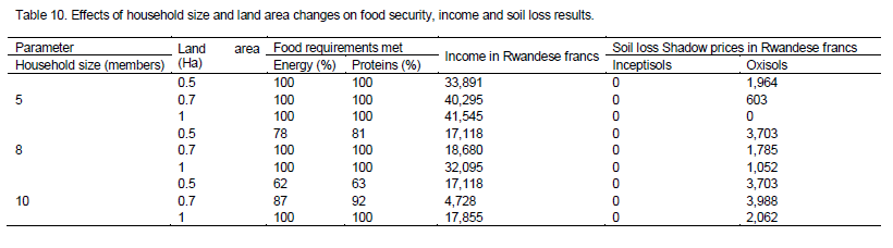
Table 10 indicates the effects of household and land size on food security, income and soil loss results. According to the model, for the majority of farm households, it is possible to meet the WHO nutritional requirements. However, households with 8 members and a farm size of 0.5 ha and household of 10 members with farm size of 0.5 ha and 0.7 ha are not able to secure the WHO energy requirements. Therefore, calorie requirements were lowered (Table 10) until a feasible solution was reached. However, from Table 10 it can be seen that a household with 5 members and a farm size of either 0.5, 0.7 or 1 ha can obtain a high income and that soil loss has relatively little economic impact. This is in accordance with the family planning policy of Rwanda Government which promotes a fertility rate less than 4 children per woman. Indeed, for a household of 5 members even with the lowest farm size (0.5 ha) considered, it is possible to secure the WHO’ s recommended level of calories and proteins, and additionnally get a relatively high income. Table 10 highlights the fact that with more people having less land food security cannot be achieved and soil loss has a high economic impact at least for the marginal land with Oxisols. This finding seems to contradict the conclusion made by Tiffen et al. (1994). In their study conducted, in Machakos region in Kenya, they asserted that  population  growth  has  a  positive impact on the economic development. Contrary to the findings of Tiffen et al. (1994): rather than saying “More people, less erosion”, our findings indicate that fewer people leads to little economic impact of soil erosion and enough food for each household. However, these differences have to be distinguished by keeping in mind that the farm household model is a yearly based model and under low farming inputs while Tiffen et al. (1994) examined interactions of people and environment over a period of sixty years in association with intensive farming systems.

 

 

In this article, a bio-economic farm model has been presented that can be applied for a typical farm household and be used to simulate the impact of family size, farm size, and soil erosion on farm production and food security. The bio-economic farm household model was developed by using a mathematical modelling approach. Here, some of the important underlying assumptions are discussed.

 

Capturing subsistence farming in the model

 

In this paper, the authors did not consider the option of purchasing food. Considering the option of purchasing food for the current typical farm with very low inputs and a farming fully focussed on subsistence would not represent the reality of livelihoods of farmers in the east region of Rwanda. However, this option may be appropriate for the livestock farms (they are large farms of more than 3 ha) who are also found in the region, but are less important in terms of total population in the province. Castaño (2001) and Laborte et al. (2009) have considered the option of purchasing food in their respective farm household models in the contexts of semi-subsistence and subsistence farming. Livestock activities, however, have been considered in their models. These activities are missing for the typical farm household considered in our model. It is known that livestock activities may constitute another source of income and a form of savings, which may then allow farmers to purchase food when necessary.

 

Subsistence farmers used the food produced from their own farms to feed their families. However, during the period of starvation, subsistence farmers may consider the option of purchasing food. In this article, the year considered in the model is assumed to be ‘normal’ where farmers do not have to face starvation due to droughts or inundation. Moreover, although that we did not program the option of purchasing food in our model, which would give more flexibility to household, we have dealt this in a flexible way in the sense that we relaxed the food constraints at the moment when the model was not able to produce enough food (Table 10).

 

Risks consideration in the model

 

In this article, the authors have used  the method of standard deviation of the gross margin to compute risk instead of a safety-first approach, including Target-MOTAD. The model somehow makes already use of the safety-first approach principle in the sense that food requirements are explicitly formulated as constraints.3.5.

 

Maximizing the objective function in the model

 

In this paper, we have assumed that the farmer is pursuing one objective that is to maximize the expected utility. Thus, the expected utility is the objective function and this is maximized. Subsistence farming characterizes most of the agricultural production of rural developing countries. Mishev et al. (2002) have stated that subsistence farmers are prone to maximize utility functions. Castaño (2001) and Laborte et al. (2009) have conducted empirical studies wherein the objective function was to maximize utility defined as discretionary income, in Andean hillside farms of Columbia and northern Philippines, respectively. Discretionary income is defined as income available for spending after essential expenses have been made. The farmer is assumed to maximise one objective function, which is the expected utility defined as discretionary income minus the risk premium. However, subsistence farmers may, also pursuit several objectives as Berkhout et al. (2010) have shown that there is heterogeneity in the farmer goals and preferences, in relation to the role of farm enterprise. Therefore, not considering all objectives of the farmer in the modelling approach, may lead to the results that differ from the reality. Given that the different approaches to capture the objective (s) of the farmer have their own limitations, the results should be analysed with respect to the particular farming system (Van Calker, 2004).

In this paper, a bio-economic model was developed to analyse the impacts of family planning, land consolidation and soil erosion on farm production and food security on a typical farm in Rwanda and on other farm types.

 

The results of the model show that a higher availability of good land increases farm income, whereas a higher availability of marginal land has slight impact on income. Considering that soil erosion is a restricting factor on marginal land, preserving soils against erosion would release more marginal land and increase food production. Farm household income would also benefit from better off-farm employment opportunities.

 

Household size and land area changes have a large impact on food security, income and soil loss. Our model results suggest that most farm households can satisfy the WHO minimum  nutritional  requirements. However, with more people and less land, it is difficult to fulfill the WHO’s energy and proteins requirements. Households with a large family size and small land area cannot ensure their food security. The model results show that a household with 8 members and a farm size of 0.5 ha and a household of 10 members with farm size of 0.5 ha and 0.7 ha are not able to secure the WHO energy requirements. Also, results show that soil loss has in those situations a relatively high economic impact. However, households with the lowest person: land ratio easily secure their food security and soil loss has relatively little economic impact for those households.

 

The outcome of the model supports the Rwanda policy on family planning which intends to encourage every woman to have a human reproduction rate below 4. However, the land policy to encourage farmers with a total land area below 1 ha either to consolidate their land or to quit farming is not supported by the results. Our results show that a household of 5 members with a farm size of at least 0.5 ha is able to comply with the minimum food security requirements and to get a relatively high income; additionnally, the soil loss has little economic impact. In the context of Rwanda with a rapidly growing population, a minimum area of 0.5 ha instead of 1 ha should be considered (for the time being).

 

Moreover, policy makers should target adoption of technologies that reduce land degradation and risks to further improve food security. 

The authors have not declared any conflict of interest.

The authors are grateful to the reviewer and the editor who have greatly contributed to improve of this paper.

REFERENCES

Acs S, Berentsen PMB, Huirne RBM (2009). Effect of yield and price risk on conversion from conventional to organic farming. Austr. J. Agric. Resourc. Econ. 3:393–411.